These are simple examples, which explains how to run simple problems for the computational homogenisation of representative volume element (RVE). The RVE boundary conditions (including linear displacement, uniform traction and periodic) are implemented in a generalized manner using the procedure given in [1]. The homogenised or effective stiffness matrices are calculated, which gives the relation between macro-strain and macro-stress.
How to cite us?

Theoretical background
Detailed theoretical background and implementation of the RVE boundary condition, while using hierarchic finite element [2] can be found in the attached pdf file and can be downloaded from this link.
Numerical examples
The following numerical examples are considered for the computational homogensation.
homogeneous linear elastic material
Before applying the RVE boundary conditions to the actual two-phase composite materials. The implementation is validated by an RVE consisting of linear-elastic homogeneous cube with unit dimensions. Mesh file for the RVE with boundary conditions and material properties is created with the following CUBIT journal file. Same mesh file is used for all three types of boundary conditions including linear displacement, traction and periodic.
#!python
#To create RVE for all the three type of boundary conditions, i.e. (Linear dispacemet, traction and periodic)
cubit.cmd('new')
cubit.cmd('brick x 1 y 1 z 1')
interval=4;
str1='block 1 ' +' volume 1'; cubit.cmd(str1)
str1='block 1 ' +' name "MAT_ELASTIC"'; cubit.cmd(str1)
cubit.cmd('block 1 attribute count 2')
Elastic=['200', '0.3']
for i in range(0, 2):
str1='block 1 attribute index ' + str(i+1) +' '+Elastic[i]; cubit.cmd(str1)
str1='surface 4 interval '+str(interval); cubit.cmd(str1)
cubit.cmd('surface 4 scheme trimesh')
cubit.cmd('mesh surface 4')
cubit.cmd('surface 6 scheme copy source surface 4 source vertex 4 target vertex 1 source curve 9 target curve 10 nosmoothing')
cubit.cmd('mesh surface 6')
str1='surface 1 interval '+str(interval); cubit.cmd(str1)
cubit.cmd('surface 1 scheme trimesh')
cubit.cmd('mesh surface 1')
cubit.cmd('surface 2 scheme copy source surface 1 source vertex 4 target vertex 7 source curve 3 target curve 7 nosmoothing')
cubit.cmd('mesh surface 2')
str1='surface 3 interval '+str(interval); cubit.cmd(str1)
cubit.cmd('surface 3 scheme trimesh')
cubit.cmd('mesh surface 3')
cubit.cmd('surface 5 scheme copy source surface 3 source vertex 7 target vertex 8 source curve 9 target curve 11 nosmoothing')
cubit.cmd('mesh surface 5')
cubit.cmd('volume 1 scheme tetmesh')
cubit.cmd('mesh volume 1')
cubit.cmd('sideset 101 surface 2 3 4') # all -ve boundary surfaces
cubit.cmd('sideset 102 surface 1 5 6') # all +ve boundary surfaces
cubit.cmd('sideset 103 surface 1 2 3 4 5 6') # all boundary surfaces
cubit.cmd('save as "/Users/zahur/Documents/moFEM/mofem-cephas/mofem_v0.2/users_modules/homogenisation/meshes/Cube.cub" overwrite')
The following material properties are used in this case
- Young’s modulus = 200
- Poisson's ratio = 0.3
The analysis procedure in this case consists of the following command, the output of which is full homogenised stiffness matrix
mpirun -np 1 ./rve_mechanical -my_file Cube.cub -ksp_type fgmres -pc_type lu -pc_factor_mat_solver_package mumps -ksp_monitor -my_order 1 -my_bc_type disp
Notes:
- Approximation order can be set using -my_order.
- Mesh file can be specified using -my_file.
- Number of processor can be specified using -np.
- The type of boundary condiitons can be specified using -my_bc_type (disp, trac, periodic)
Macro strain vector is written as
\[ \overline{\boldsymbol{\varepsilon}}=\left[\begin{array}{cccccc}\overline{\varepsilon}_{xx} & \overline{\varepsilon}_{yy} & \overline{\varepsilon}_{zz} & 2\overline{\varepsilon}_{xy} & 2\overline{\varepsilon}_{yz} & 2\overline{\varepsilon}_{zx}\end{array}\right]^{T} \]
A sample mesh and corresponding x-displacement contours for a macro-strain of [1.0, 0.0, 0.0, 0.0, 0.0, 0.0] are shown in the following figure.
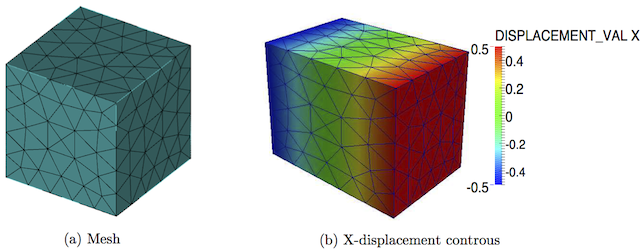
Mesh and x-contours of displacement for a linear-elastic homogeneous cube
The homogenised stiffness matrices calculated using all the three types of boundary conditions are shown in the following Table. The homogenized stiffness matrices for the three type of boundary conditions are also compared with one calculated directly from the Hooke's law, which is also given in the same table. It is clear from the Table, that the homogenised stiffness matrix calculated for a homogeneous material is the same for all three types of boundary conditions and is also the same as calculated directly from the Hooke's law. In the following, the code is used for a more complex case, i.e. a unidirectional fibre reinforced composites and textile composite RVEs.
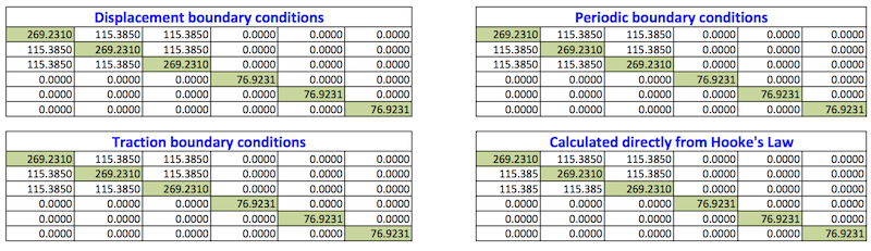
Homogenised stiffness matrices for linear-elastic homogeneous cube
Unidirectional fibre reinforced composites
The second example consists of unidirectional fibre reinforced composites, the geometry for which is given in the following figure. Periodic mesh is created for the RVE, in which, e.g. for every nodes on the positive x-face there is a node on the negative x-face with same y and z coordinates. In this example matrix is considered as isotropic and yarn is considered as transversely isotropic materials. The following CUBIT journal file is used to create the geometry with boundary conditions and material properties. The material properties used for the matrix and fibres are given as
Matrix:
- Young’s modulus = 3.5 GPa
- Poisson's ratio = 0.35
Fibres:
- Young’s modulus in transverse direction E_p = 35 GPa
- Poisson's ratio in transverse direction v_p = 0.26
- Young’s modulus in fibre direction E_z = 70 GPa
- Poisson's ratio in fibre direction v_pz = 0.26
- Shear modulus in the fibre direction G_pz = 17.5 GPa
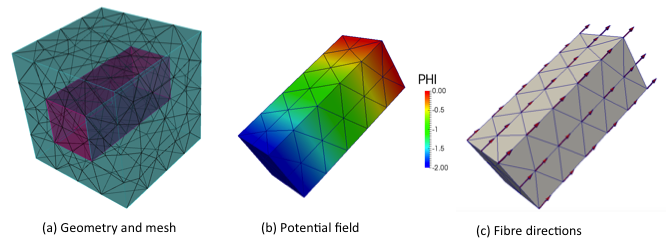
Geometry, potential field and fibres directions for unidirectional fibre reinforced composites
#!python
#To create RVE for all the three type of boundary conditions, i.e. (Linear dispacemet, traction and periodic)
cubit.cmd('new')
autofactor=7;
#=============================================================
#Geometry
#=============================================================
cubit.cmd('brick x 1 y 1 z 1')
cubit.cmd('brick x 1 y 0.4 z 0.4')
cubit.cmd('subtract volume 2 from volume 1 keep')
cubit.cmd('delete volume 1')
cubit.cmd('imprint volume 2 3')
cubit.cmd('merge volume 2 3')
#=============================================================
#Periodic mesh
#=============================================================
cubit.cmd('surface 20 scheme trimesh')
str1='surface 20 size auto factor '+str(autofactor); cubit.cmd(str1)
cubit.cmd('mesh surface 20')
cubit.cmd('surface 22 scheme copy source surface 20 source vertex 27 target vertex 26 source curve 47 target curve 48 nosmoothing')
cubit.cmd('mesh surface 22')
cubit.cmd('surface 10 scheme trimesh')
str1='surface 10 size auto factor '+str(autofactor); cubit.cmd(str1)
cubit.cmd('mesh surface 10')
cubit.cmd('surface 12 scheme copy source surface 10 source vertex 11 target vertex 10 source curve 23 target curve 24 nosmoothing')
cubit.cmd('mesh surface 12')
cubit.cmd('surface 17 scheme trimesh')
str1='surface 17 size auto factor '+str(autofactor); cubit.cmd(str1)
cubit.cmd('mesh surface 17')
cubit.cmd('surface 18 scheme copy source surface 17 source vertex 26 target vertex 29 source curve 38 target curve 44 nosmoothing')
cubit.cmd('mesh surface 18')
cubit.cmd('surface 19 scheme trimesh')
str1='surface 19 size auto factor '+str(autofactor); cubit.cmd(str1)
cubit.cmd('mesh surface 19')
cubit.cmd('surface 21 scheme copy source surface 19 source vertex 28 target vertex 27 source curve 45 target curve 47 nosmoothing')
cubit.cmd('mesh surface 21')
str1='volume all size auto factor '+str(autofactor); cubit.cmd(str1)
cubit.cmd('volume all scheme tetmesh')
cubit.cmd('mesh volume all')
#=============================================================
#Defining blocks for elastic, transversely-isotropic and potential flow problems
#=============================================================
vol=['3', '2','2']
mat=['MAT_ELASTIC_1','MAT_ELASTIC_TRANSISO_1','PotentialFlow_1']
for i in range(0, 3):
cubit.cmd('set duplicate block elements on')
str1='block ' + str(i+1) +' volume '+vol[i]; cubit.cmd(str1)
str1='block ' + str(i+1) +' name "'+mat[i] + '"'; cubit.cmd(str1)
#=============================================================
#Material properties for matrix part
#=============================================================
cubit.cmd('block 1 attribute count 2')
Em=3.5e3; Enu=0.3; #giga to mega as we used dimension in mm
Elastic=[str(Em), str(Enu)]
for i in range(0, 2):
str1='block 1 attribute index ' + str(i+1) +' '+Elastic[i]; cubit.cmd(str1)
#=============================================================
#Material properties for fibres
#=============================================================
#to use as isotropic
#cubit.cmd('block 2 attribute count 5')
#Ep=Em; Ez=Em; nup=Enu; nupz=Enu; Gzp=Em/(2*(1+Enu));
cubit.cmd('block 2 attribute count 5')
#Ep=40e3; Ez=230e3; nup=0.26; nupz=0.26; Gzp=24e3;
Ep=10*Em; Ez=20*Em; nup=0.26; nupz=0.26; Gzp=5*Em;
#Ep=2*Em; Ez=5*Em; nup=0.26; nupz=0.26; Gzp=2*Em;
TransIso=[str(Ep), str(Ez), str(nup), str(nupz), str(Gzp)]
for i in range(0, 5):
str1='block 2 attribute index ' + str(i+1) +' '+TransIso[i]; cubit.cmd(str1)
#=============================================================
#Material properties for interface between fibres and matrix
#=============================================================
alpha_interf=500
cubit.cmd('set duplicate block elements on')
str1='block 7 surface 23 26 29 32'; cubit.cmd(str1)
str1='block 7 name "MAT_INTERF_1"'; cubit.cmd(str1)
cubit.cmd('block 7 attribute count 4')
str1='block 7 attribute index 1 '+str(alpha_interf); cubit.cmd(str1) #now we use 4 parameters for interface
str1='block 7 attribute index 2 '+str(0.0); cubit.cmd(str1)
str1='block 7 attribute index 3 '+str(0.0); cubit.cmd(str1)
str1='block 7 attribute index 4 '+str(0.0); cubit.cmd(str1)
#=============================================================
#Defining interfaces
#=============================================================
Interface=['7', '8','9','11']
for i in range(0, 4):
str1='sideset ' + str(i+1) +' surface '+Interface[i]; cubit.cmd(str1)
str1='sideset ' + str(i+1) +' name "interface'+str(i+1); cubit.cmd(str1)
#=============================================================
#Defining pressures for potential flow problem
#=============================================================
Pres=['10', '12']; count=0; count1=len(Interface);
for i in range(0, 1):
str1='create pressure '+str(count+1)+' on surface '+str(Pres[count])+' magnitude 1'; cubit.cmd(str1)
str1='create pressure '+str(count+2)+' on surface '+str(Pres[count+1])+' magnitude -1'; cubit.cmd(str1)
str1='sideset '+str(count1+1)+' name "PressureIO_' + str(i+1) + '_1"'; cubit.cmd(str1)
str1='sideset '+str(count1+2)+' name "PressureIO_' + str(i+1) + '_2"'; cubit.cmd(str1)
count=count+2; count1=count1+2;
#=============================================================
#Definign zero proessrues for potential flow problem (This should be of the same order as PotentialFlow blocks )
#=============================================================
zeroPressureNode=[1]
for i in range(0, 1):
str1='nodeset ' + str(i+1) + ' node ' + str(zeroPressureNode[i]); cubit.cmd(str1)
str1='nodeset ' + str(i+1)+' name "ZeroPressure_' + str(i+1)+ '"'; cubit.cmd(str1)
#=============================================================
#Defining surfaces for dispacement, traction and periodic boundary conditions
#=============================================================
cubit.cmd('sideset 101 surface 20 10 19 18') # all -ve boundary surfaces
cubit.cmd('sideset 102 surface 21 17 22 12') # all +ve boundary surfaces
cubit.cmd('sideset 103 surface 20 10 19 18 21 17 22 12') # all boundary surfaces
cubit.cmd('save as "/Users/zahur/Documents/moFEM/mofem-cephas/mofem_v0.2/users_modules/homogenisation/meshes/Cube_RVE_with_reinforcement.cub" overwrite')
The fibre direction, required for the transversely isotropic material model is calculated by solving a potential flow problem across the fibre. The analysis procedure in this example consists of running a potential flow problem followed by actual computational homogenisation calculation. The commands used for this example is given as follows, the output of which is full homogenised stiffness matrix for linear displacement, uniform traction and periodic boundary conditions cases.
mpirun -np 1 ./rve_fibre_directions -my_file Cube_RVE_with_reinforcement.cub -ksp_type fgmres -pc_type lu -pc_factor_mat_solver_package superlu_dist -ksp_monitor -my_order 1
mpirun -np 1 ./rve_mechanical -my_file solution_RVE.h5m -ksp_type fgmres -pc_type lu -pc_factor_mat_solver_package mumps -ksp_monitor -my_order 1 -my_bc_type disp
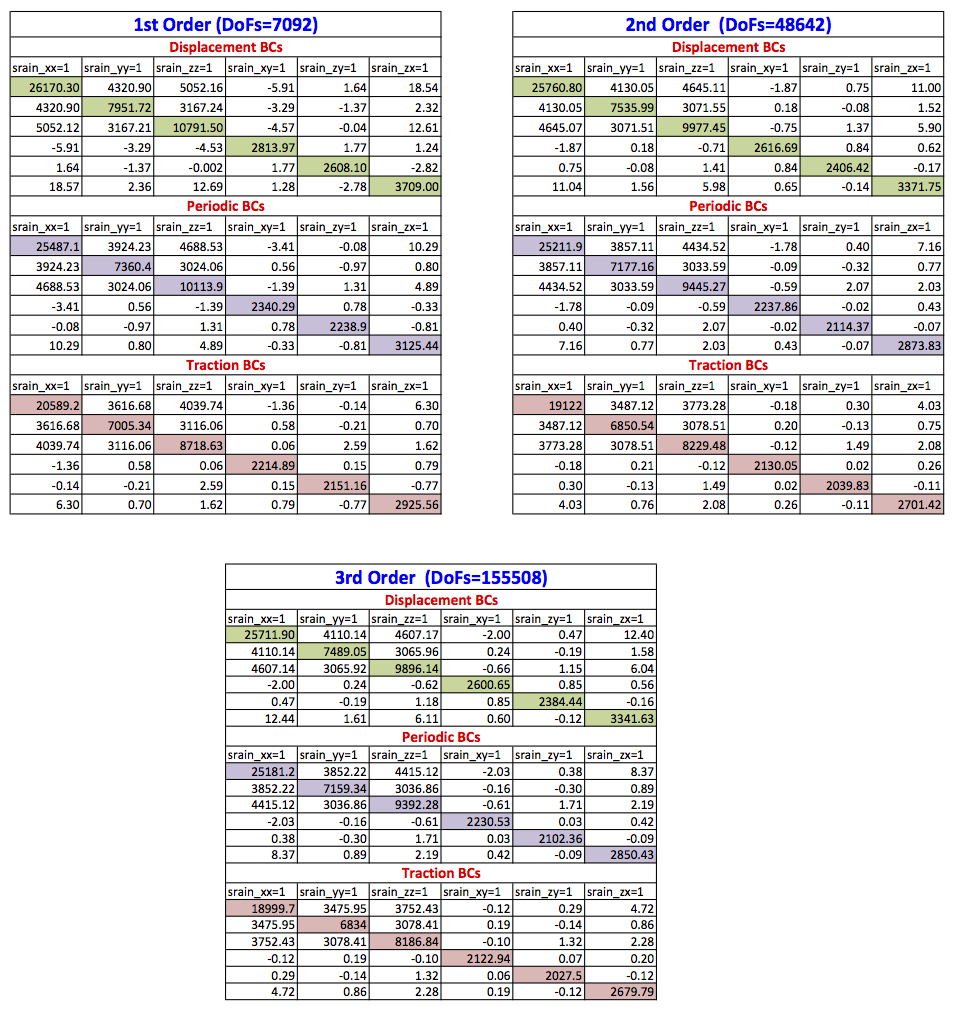
The output of the potential flow, including potential filed and calculated fibre direction are also given in the above figure. The full-homogenised stiffness matrices calculated for displacement, periodic and traction boundary conditions for 1st, 2nd and 3rd order of approximation are given in the following table.
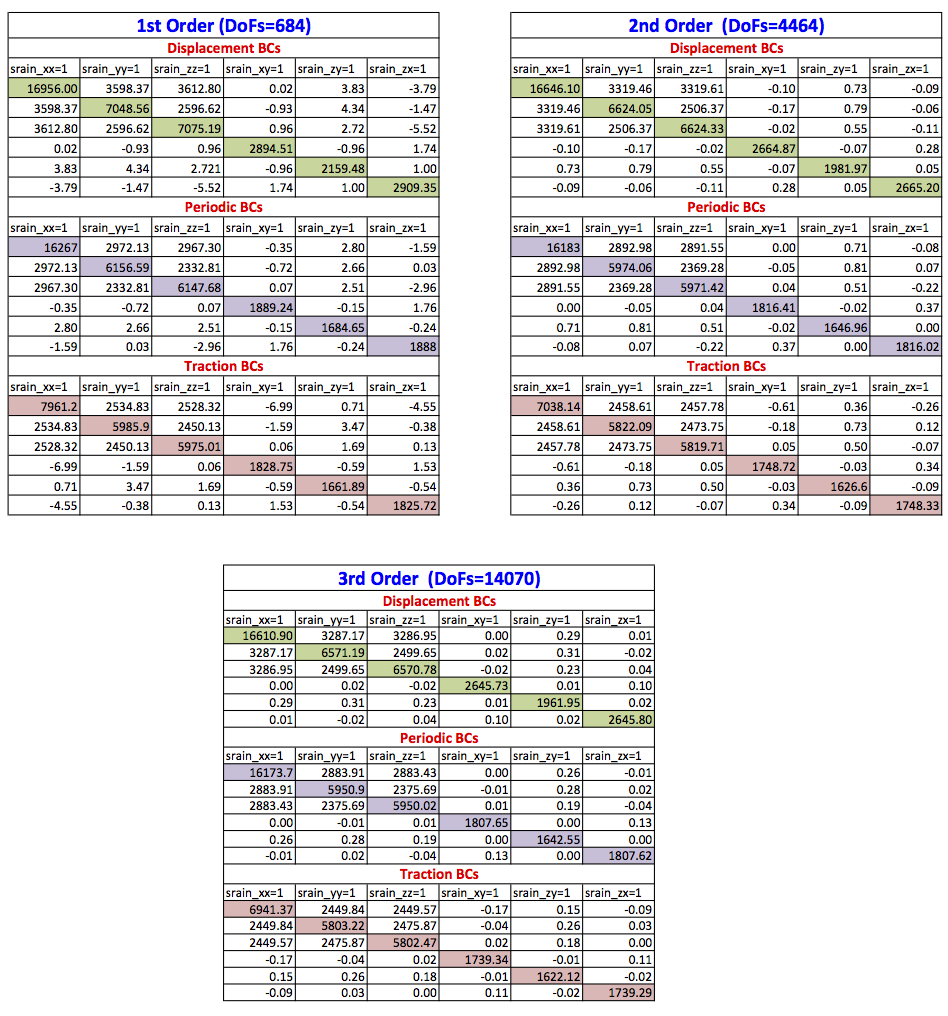
Homogenised stiffness matrix for 1st, 2nd and 3rd order of approximations for unidirectional fibre reinforced composites
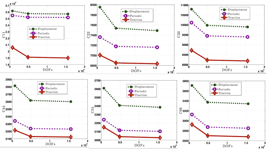
Furthermore comparison and convergence of C11, C22, C33, C44, C55 and C66 for all the three types of boundary conditions are also given in the following figure. It is clear that as expected response for the periodic boundary condition case lies between the traction and displacement boundary conditions cases. Moreover Convergence can be observed in all Cs as we increase the order of approximation from 1st to 3rd.
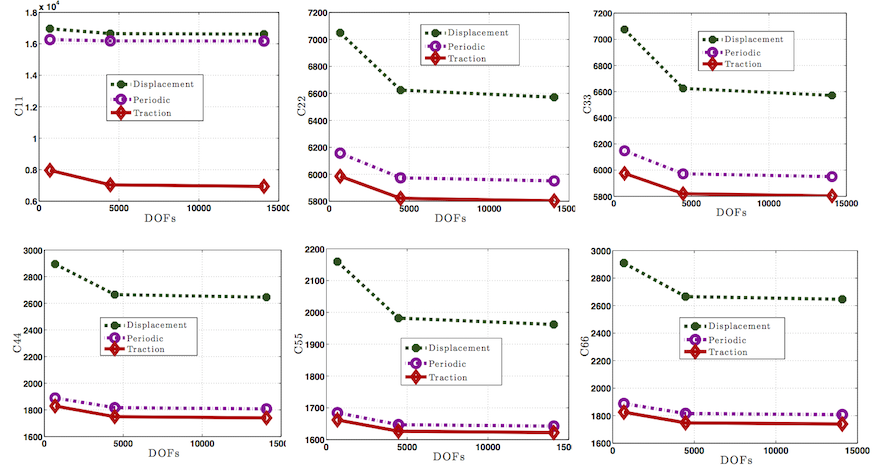
Figure 6. Comparison of C11, C22, C33, C44, C55 and C66 for displacement, traction and periodic boundary conditions for unidirectional fibre reinforced composites
Textile reinforced composites (a)
In this case a more complicated textile RVE is considered [3] consisting of matrix and textile fibres imbedded in matrix. Elliptical cross sections and cubic splines are used to model the cross-sections and paths of the fibre. Different parameters defining the RVE geometry are given in the following figure.
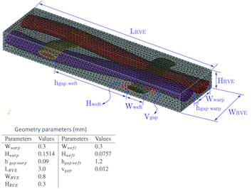
RVE geometry for the textile composite
The CUBIT journal file required to generate the input model is given as follows (same file is used for all the three types of boundary conditions):
#!python
#This scrip will create RVE including fibres and matrix, which can be used for all
#three type of boundary conditions including dispalcement, traction and periodic.
cubit.cmd('new')
#=============================================================
#Geometry Input parametrs
#=============================================================
W_wrap=0.3; H_wrap=0.1514; hgap_wrap=0.09
W_weft=0.3; H_weft=0.0757; hgap_weft=1.2
L_RVE=3.0; W_RVE=0.8; H_RVE=0.3;
Vgap=0.012
s_weft=hgap_weft+W_weft; s_wraf=hgap_wrap+W_wrap
T=(H_weft/2+H_wrap/2)/2+Vgap
L_RVE=2*s_weft; W_RVE=2*s_wraf; H_RVE=0.3;
#=============================================================
#Create vartices for splines to create splines
#=============================================================
coordx=-22.5*s_weft; coordy=T; coordz=0;
for i in range(0, 48):
if i % 2 == 0:
str1='create vertex ' + str(coordx) +' '+str(coordy)+' '+str(coordz)+' color' ; coordx=coordx+s_weft;
cubit.cmd(str1)
if i % 2 == 1:
str1='create vertex ' + str(coordx) +' '+str(-coordy)+' '+str(coordz)+' color' ; coordx=coordx+s_weft;
cubit.cmd(str1)
coordx=-22.5*s_weft; coordy=-T; coordz=s_wraf;
for i in range(0, 48):
if i % 2 == 0:
str1='create vertex ' + str(coordx) +' '+str(coordy)+' '+str(coordz)+' color' ; coordx=coordx+s_weft;
cubit.cmd(str1)
if i % 2 == 1:
str1='create vertex ' + str(coordx) +' '+str(-coordy)+' '+str(coordz)+' color' ; coordx=coordx+s_weft;
cubit.cmd(str1)
coordx=-0.5*s_weft; coordy=-T; coordz=-22*s_wraf;
for i in range(0, 48):
if i % 2 == 0:
str1='create vertex ' + str(coordx) +' '+str(coordy)+' '+str(coordz)+' color' ; coordz=coordz+s_wraf;
cubit.cmd(str1)
if i % 2 == 1:
str1='create vertex ' + str(coordx) +' '+str(-coordy)+' '+str(coordz)+' color' ; coordz=coordz+s_wraf;
cubit.cmd(str1)
coordx=0.5*s_weft; coordy=T; coordz=-22*s_wraf;
for i in range(0, 48):
if i % 2 == 0:
str1='create vertex ' + str(coordx) +' '+str(coordy)+' '+str(coordz)+' color' ; coordz=coordz+s_wraf;
cubit.cmd(str1)
if i % 2 == 1:
str1='create vertex ' + str(coordx) +' '+str(-coordy)+' '+str(coordz)+' color' ; coordz=coordz+s_wraf;
cubit.cmd(str1)
#=============================================================
#Joint vertices to create splines
#=============================================================
Tvertices=48;
vertices=range(1,Tvertices+1); count1=0;
for i in range(0, 4):
str1='create curve spline vertex '
for j in range(0, 48):
str1=str1+' '+ str(count1+vertices[j])
cubit.cmd(str1); count1=count1+48;
#=============================================================
#Creating fibers with elliptical cross sections
#=============================================================
cubit.cmd('create planar surface with plane normal to curve 1 distance 0 from vertex 1')
str1='create curve location vertex 1 direction curve 8 length '+ str(W_wrap/2); cubit.cmd(str1)
str1='create curve location vertex 1 direction curve 7 length '+str(H_wrap/2); cubit.cmd(str1)
cubit.cmd('create surface ellipse vertex 198 200 1')
cubit.cmd('sweep surface 2 along curve 1')
cubit.cmd('create planar surface with plane normal to curve 2 distance 0 from vertex 49')
str1='create curve location vertex 49 direction curve 17 length '+ str(W_wrap/2); cubit.cmd(str1)
str1='create curve location vertex 49 direction curve 16 length '+str(H_wrap/2); cubit.cmd(str1)
cubit.cmd('create surface ellipse vertex 208 210 49')
cubit.cmd('sweep surface 6 along curve 2')
cubit.cmd('create planar surface with plane normal to curve 3 distance 0 from vertex 97')
str1='create curve location vertex 97 direction curve 24 length '+ str(W_weft/2); cubit.cmd(str1)
str1='create curve location vertex 97 direction curve 23 length '+str(H_weft/2); cubit.cmd(str1)
cubit.cmd('create surface ellipse vertex 218 220 97')
cubit.cmd('sweep surface 10 along curve 3')
cubit.cmd('create planar surface with plane normal to curve 4 distance 0 from vertex 145')
str1='create curve location vertex 145 direction curve 33 length '+ str(W_weft/2); cubit.cmd(str1)
str1='create curve location vertex 145 direction curve 32 length '+str(H_weft/2); cubit.cmd(str1)
cubit.cmd('create surface ellipse vertex 228 230 145')
cubit.cmd('sweep surface 14 along curve 4')
#=============================================================
#Deletion of remaining free vertices, curves and bodies
#=============================================================
cubit.cmd('delete vertex all')
cubit.cmd('delete curve all')
cubit.cmd('delete body 7 3 5 1')
#=============================================================
#Create matrix and imprint and merge fibres and matrix to create common surfaces
#=============================================================
str1='brick x '+str(L_RVE)+' y '+str(H_RVE)+' z '+str(W_RVE); cubit.cmd(str1)
str1='move Volume '+str(9)+' x '+str(0)+' y '+str(0)+' z '+str(s_wraf/2); cubit.cmd(str1)
cubit.cmd('intersect volume all keep')
cubit.cmd('delete volume 6 2 8 4')
cubit.cmd('subtract volume 10 11 12 13 from volume 9 keep')
cubit.cmd('delete volume 9')
cubit.cmd('imprint volume 10 11 12 13 14')
cubit.cmd('merge volume 10 11 12 13 14')
#=============================================================
#Meshing negative x, y and z face of the RVE and coping the same to its positive faces
#=============================================================
cubit.cmd('group 1 add surface 42 27 24')
cubit.cmd('group "g2" add surface 44 25 28')
cubit.cmd('group "g3" add surface 39 30 33')
cubit.cmd('group "g4" add surface 31 40 34')
cubit.cmd('group "g5" add surface 43')
cubit.cmd('group "g6" add surface 41')
cubit.cmd('surface 42 27 24 size auto factor 6')
cubit.cmd('surface 42 27 24 scheme trimesh')
cubit.cmd('mesh surface 42 27 24')
cubit.cmd('surface 28 25 44 scheme mirror source surface 27 24 42 source vertex 263 target vertex 262 nosmoothing')
cubit.cmd('mesh surface 28 25 44')
cubit.cmd('surface 39 30 33 size auto factor 5')
cubit.cmd('surface 39 30 33 scheme trimesh')
cubit.cmd('mesh surface 39 30 33')
cubit.cmd('surface 31 34 40 scheme mirror source surface 30 33 39 source vertex 257 target vertex 262 nosmoothing')
cubit.cmd('mesh surface 31 34 40')
cubit.cmd('surface 43 scheme trimesh')
cubit.cmd('mesh surface 43')
cubit.cmd('surface 41 scheme mirror source surface 43 source vertex 259 target vertex 260 nosmoothing')
cubit.cmd('mesh surface 41')
#=============================================================
#Mesh volume
#=============================================================
cubit.cmd('volume all scheme Tetmesh')
cubit.cmd('mesh volume all')
#=============================================================
#Defining blocks for elastic, transversely-isotropic and potential flow problems
#=============================================================
vol=['14', '10,11,12,13','10', '11', '12', '13']
mat=['MAT_ELASTIC_1','MAT_ELASTIC_TRANSISO_1','PotentialFlow_1','PotentialFlow_2','PotentialFlow_3','PotentialFlow_4']
for i in range(0, 6):
cubit.cmd('set duplicate block elements on')
str1='block ' + str(i+1) +' volume '+vol[i]; cubit.cmd(str1)
str1='block ' + str(i+1) +' name "'+mat[i] + '"'; cubit.cmd(str1)
#=============================================================
#Material properties for matrix part
#=============================================================
cubit.cmd('block 1 attribute count 2')
Em=3.5e3; Enu=0.3; #gig to mega as we used dimension in mm
Elastic=[str(Em), str(Enu)]
for i in range(0, 2):
str1='block 1 attribute index ' + str(i+1) +' '+Elastic[i]; cubit.cmd(str1)
#=============================================================
#Material properties for fibres
#=============================================================
#to use as isotropic
#cubit.cmd('block 2 attribute count 5')
#Ep=Em; Ez=Em; nup=Enu; nupz=Enu; Gzp=Em/(2*(1+Enu));
cubit.cmd('block 2 attribute count 5')
#Ep=40e3; Ez=230e3; nup=0.26; nupz=0.26; Gzp=24e3;
Ep=10*Em; Ez=20*Em; nup=0.26; nupz=0.26; Gzp=5*Em;
#Ep=2*Em; Ez=5*Em; nup=0.26; nupz=0.26; Gzp=2*Em;
TransIso=[str(Ep), str(Ez), str(nup), str(nupz), str(Gzp)]
for i in range(0, 5):
str1='block 2 attribute index ' + str(i+1) +' '+TransIso[i]; cubit.cmd(str1)
#=============================================================
#Material properties for interface between fibres and matrix
#=============================================================
alpha_interf=500
cubit.cmd('set duplicate block elements on')
str1='block 7 surface 23 26 29 32'; cubit.cmd(str1)
str1='block 7 name "MAT_INTERF_1"'; cubit.cmd(str1)
cubit.cmd('block 7 attribute count 4')
str1='block 7 attribute index 1 '+str(alpha_interf); cubit.cmd(str1) #now we use 4 parameters for interface
str1='block 7 attribute index 2 '+str(0.0); cubit.cmd(str1)
str1='block 7 attribute index 3 '+str(0.0); cubit.cmd(str1)
str1='block 7 attribute index 4 '+str(0.0); cubit.cmd(str1)
#=============================================================
#Defining interfaces
#=============================================================
Interface=['23', '26','29','32']
for i in range(0, 4):
str1='sideset ' + str(i+1) +' surface '+Interface[i]; cubit.cmd(str1)
str1='sideset ' + str(i+1) +' name "interface'+str(i+1); cubit.cmd(str1)
#=============================================================
#Defining pressures for potential flow problem
#=============================================================
Pres=['24', '25','27','28','30','31','33','34']; count=0; count1=len(Interface);
for i in range(0, 4):
str1='create pressure '+str(count+1)+' on surface '+str(Pres[count])+' magnitude 1'; cubit.cmd(str1)
str1='create pressure '+str(count+2)+' on surface '+str(Pres[count+1])+' magnitude -1'; cubit.cmd(str1)
str1='sideset '+str(count1+1)+' name "PressureIO_' + str(i+1) + '_1"'; cubit.cmd(str1)
str1='sideset '+str(count1+2)+' name "PressureIO_' + str(i+1) + '_2"'; cubit.cmd(str1)
count=count+2; count1=count1+2;
#=============================================================
#Defining surfaces for dispacement, traction and periodic boundary conditions
#=============================================================
cubit.cmd('sideset 101 surface 41 31 34 40 42 27 24') # all -ve boundary surfaces for periodic boundary conditions
cubit.cmd('sideset 102 surface 43 30 33 39 25 44 28') # all +ve boundary surfaces for periodic boundary conditions
cubit.cmd('sideset 103 surface 41 31 34 40 42 27 24 43 30 33 39 25 44 28') # all boundary surfaces
#To check for indiviual side for inserstion of prisms of any problem
#cubit.cmd('sideset 101 surface 42 27 24')
#cubit.cmd('sideset 102 surface 25 44 28')
#cubit.cmd('sideset 101 surface 41')
#cubit.cmd('sideset 102 surface 43')
#cubit.cmd('sideset 101 surface 31 34 40')
#cubit.cmd('sideset 102 surface 30 33 39')
#cubit.cmd('sideset 101 surface 40')
#cubit.cmd('sideset 102 surface 39')
#=============================================================
#Definign zero proessrues for potential flow problem (This should be of the same order as PotentialFlow blocks )
#=============================================================
zeroPressureNode=[140, 106, 279, 272]
for i in range(0, 4):
str1='nodeset ' + str(i+1) + ' node ' + str(zeroPressureNode[i]); cubit.cmd(str1)
str1='nodeset ' + str(i+1)+' name "ZeroPressure_' + str(i+1)+ '"'; cubit.cmd(str1)
#=============================================================
#Saving input RVE file
#=============================================================
cubit.cmd('save as "/Users/zahur/Documents/moFEM/mofem-cephas/mofem_v0.2/users_modules/homogenisation/meshes/Textile_RVE_TransIso.cub" overwrite')
Similar to the previous unidirectional fibre reinforced composites example, matrix and fibres are considered as isotropic and transversely isotropic materials respectively with the same material properties. The finite element mesh (periodic) in this case consists of 4-node tetrahedral elements and is shown in following figure.
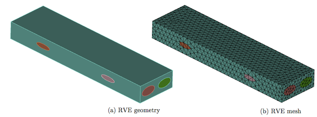
RVE geometry and corresponding mesh for the textile composite
The commands for the calculation of e.g. the first column of the homogenised stiffness matrix for the displacement, periodic and traction boundary conditions for this example is given as
mpirun -np 1 ./rve_fibre_directions -my_file Textile_RVE_TransIso.cub -ksp_type fgmres -pc_type lu -pc_factor_mat_solver_package superlu_dist -ksp_monitor -my_order 1
mpirun -np 1 ./rve_mechanical -my_file solution_RVE.h5m -ksp_type fgmres -pc_type lu -pc_factor_mat_solver_package mumps -ksp_monitor -my_order 1 -my_bc_type disp
For this example, the potential field and calculated fibres directions are shown in the following figure.
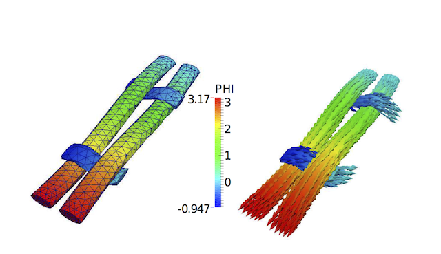
Potential field (left) and calculated fibres directions (right) for the textile composite
Finally, the full homogenised stiffness matrices (6x6) is calculated for all the three types of boundary conditions for 1st and 2nd order of approximation and is given in the following table
Homogenised stiffness matrix for 1st, 2nd and 3rd order of approximations for the textile composite
Comparison of C11, C22, C33, C44, C55 and C66 for displacement, traction and periodic boundary conditions for this example are shown in the following figure. It is clear that response for the periodic boundary conditions case lies between the displacement and traction boundary conditions cases. Convergence can also be observed in C11, C22, C33, C44, C55 and C66 as we increase the order of approximation from 1st to 3rd.
Comparison of C11, C22, C33, C44, C55 and C66 for displacement, traction and periodic boundary conditions for the textile composite
Textile reinforced composites (b)
Two RVE microstructures with plain weave fabric reinforcement [4, 5] and [4, 6] are selected to evaluate the applicability of computational homogenization scheme for textile composites, comparing with experimental and/or existing model results. These two models are named the Barbero model and the Scida model here after. The Barbero model is based on photomicrograph measurements of geometrical parameters and the Mori-Tanaka asymptotic homogenization method has been applied to predict the effective elastic parameters. The geometrical parameters of the Scida model were also obtained by photomicrography, and experiments were conducted to obtain the longitudinal and transversal Young’s moduli and the in-plane Poisson’s ratio. The geometry for this case with different parameters and fibres directions are shown in the following figures, in which 4a1 and 4a2 are the periodic length of warp and weft yarns, 2a3 is the waviness amplitude and ag1 and ag2 are spacing between adjacent warp and weft yarns respectively.
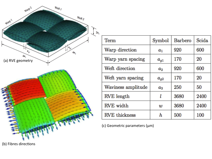
RVE geometry and potential flow for the textile composite (b) [4]
The RVE of the Barbero model has been discretized into 12148 four-node tetrahedral elements consisting of 5346 elements for the yarns and 6802 elements for the matrix, with a total of 2454 nodes, while the RVE of Scida model has been discretized into 20053 tetrahedral elements with 8101 of them for the yarns and 11952 for matrix.
The effective engineering parameters predicted by the computational homogenization method are compared with experimental and/or numerical results. The results are listed in the following table. The reference numerical results for both models are taken from [5], where both models have been analysed using the Mori-Tanaka asymptotic homogenization method. For the Scida model, the experimental results reported are from [6]. For the computational homogenization, the results for the three boundary conditions of linear displacement, periodic, and uniform traction are given in the following table. From these results it can be seen that the model predicts moduli values that are within or very near the published standard deviation.
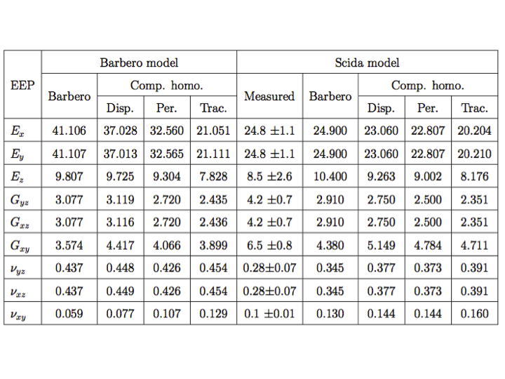
Comparison between current and reference homogenised elastic properties [4]
The CUBIT journal file used to generate the input model for Barbero RVE is given as:
#!python
#This scrip will create RVE including fibres and matrix, which can be used for all
#three type of boundary conditions including dispalcement, traction and periodic.
cubit.cmd('new')
#=============================================================
#Geometry Input parametrs
#=============================================================
a1=0.920
a2=0.920
a3=0.250
ag1=0.17
ag2=0.17
W_warp=a2-ag2/2
W_weft=a1-ag1/2
L_RVE=4*a2
W_RVE=4*a1
H_RVE=2.12*a3
dy_w=W_warp/100
dy_g=ag2/50
dx_w=W_weft/100
dx_g=ag1/50
autofactor=5;
#=============================================================
#Create vartices for splines to create splines
#=============================================================
import math
da3=0.014;
a3=a3+da3;
#---------------------
# Fill 1 path (14) top
#---------------------
coordx=-a1
coordy=-3*a2-dy_w
for i in range(0, 751):
if (i<101) or (i>150 and i<351) or (i>400 and i<601) or (i>650):
coordy=coordy+dy_w;
else:
coordy=coordy+dy_g;
coordz=a3/2*(math.sin(-math.pi*(coordy)/(2*a2)))+a3/2
str1='create vertex ' + str(coordx) +' '+str(coordy)+' '+str(coordz)+' color' ;
cubit.cmd(str1)
#---------------------
# Fill 2 path (12) top
#---------------------
coordx=a1
coordy=-3*a2-dy_w
for i in range(0, 751):
if (i<101) or (i>150 and i<351) or (i>400 and i<601) or (i>650):
coordy=coordy+dy_w;
else:
coordy=coordy+dy_g;
coordz=a3/2*(math.sin(math.pi*(coordy)/(2*a2)))+a3/2
str1='create vertex ' + str(coordx) +' '+str(coordy)+' '+str(coordz)+' color' ;
cubit.cmd(str1)
#---------------------
# Warp 1 path (2) top
#---------------------
coordy=-a2
coordx=-3*a1-dx_w
for i in range(0, 751):
if (i<101) or (i>150 and i<351) or (i>400 and i<601) or (i>650):
coordx=coordx+dx_w;
else:
coordx=coordx+dx_g;
coordz=a3/2*(math.sin(math.pi*(coordx)/(2*a1)))+a3/2
str1='create vertex ' + str(coordx) +' '+str(coordy)+' '+str(coordz)+' color' ;
cubit.cmd(str1)
#---------------------
# Warp 2 path (8) top
#---------------------
coordy=a2
coordx=-3*a1-dx_w
for i in range(0, 751):
if (i<101) or (i>150 and i<351) or (i>400 and i<601) or (i>650):
coordx=coordx+dx_w;
else:
coordx=coordx+dx_g;
coordz=a3/2*(math.sin(-math.pi*(coordx)/(2*a1)))+a3/2
str1='create vertex ' + str(coordx) +' '+str(coordy)+' '+str(coordz)+' color' ;
cubit.cmd(str1)
#=============================================================
#Joint vertices to create splines
#=============================================================
Tvertices=751;
vertices=range(1,Tvertices+1); count1=0;
for i in range(0, 4):
str1='create curve spline vertex '
for j in range(125, 626):
str1=str1+' '+ str(count1+vertices[j])
cubit.cmd(str1); count1=count1+751;
#=============================================================
#Creating yarns/inclusions with sinusoidal cross sections
#=============================================================
a3=a3-da3;
#-------------------------------------
# Fill 1 front surface top profile (1)
#-------------------------------------
coordy=3*a2
coordx=-2*a1+ag1/2-dx_w
A_coef=-a3/2*math.sin(math.pi*ag1/4/a1)-a3/2
B_coef=math.pi/(ag1-2*a1)
C_coef=-math.pi*(ag1-4*a1)/2/(ag1-2*a1)
D_coef=-a3/2*math.sin(math.pi*ag1/4/a1)+a3/2
for i in range(0, 201):
coordx=coordx+dx_w;
coordz=A_coef*math.sin(B_coef*coordx+C_coef)+D_coef
coordz=coordz+da3;
str1='create vertex ' + str(coordx) +' '+str(coordy)+' '+str(coordz)+' color' ;
cubit.cmd(str1)
dzmax=A_coef*math.sin(B_coef*(-a1)+C_coef)+D_coef
dzmin=A_coef*math.sin(B_coef*(-ag1/2)+C_coef)+D_coef
dz_f1=dzmax-dzmin
#----------------------------------------
# Fill 1 front surface bottom profile (2)
#----------------------------------------
A_coef=a3/2
B_coef=math.pi/(2*a1)
C_coef=0
D_coef=a3/2
coordy=3*a2
coordx=-2*a1+ag1/2-dx_w
for i in range(0, 201):
coordx=coordx+dx_w;
coordz=A_coef*math.sin(B_coef*coordx+C_coef)+D_coef
coordz=coordz+da3;
str1='create vertex ' + str(coordx) +' '+str(coordy)+' '+str(coordz)+' color' ;
cubit.cmd(str1)
Tvertices=201;
vertices=range(1,Tvertices+1); count1=3004;
for i in range(0, 2):
str1='create curve spline vertex '
for j in range(0, 201):
str1=str1+' '+ str(count1+vertices[j])
cubit.cmd(str1); count1=count1+201;
#-------------------------------------
# Fill 2 front surface top profile (5)
#-------------------------------------
coordy=3*a2
coordx=ag1/2-dx_w
A_coef=a3/2
B_coef=math.pi/(2*a1)
C_coef=0
D_coef=-a3/2
for i in range(0, 201):
coordx=coordx+dx_w;
coordz=A_coef*math.sin(B_coef*coordx+C_coef)+D_coef;
coordz=coordz;
str1='create vertex ' + str(coordx) +' '+str(coordy)+' '+str(coordz)+' color' ;
cubit.cmd(str1)
dzmax=A_coef*math.sin(B_coef*a1+C_coef)+D_coef
dzmin=A_coef*math.sin(B_coef*ag1/2+C_coef)+D_coef
dz_f2=dzmax-dzmin
#----------------------------------------
# Fill 2 front surface bottom profile (6)
#----------------------------------------
coordy=3*a2
coordx=ag1/2-dx_w
A_coef=-a3/2*math.sin(math.pi*ag1/4/a1)-a3/2
B_coef=math.pi/(ag1-2*a1)
C_coef=math.pi*(ag1-4*a1)/2/(ag1-2*a1)
D_coef=a3/2*math.sin(math.pi*ag1/4/a1)-a3/2
for i in range(0, 201):
coordx=coordx+dx_w;
coordz=A_coef*math.sin(B_coef*coordx+C_coef)+D_coef;
coordz=coordz;
str1='create vertex ' + str(coordx) +' '+str(coordy)+' '+str(coordz)+' color' ;
cubit.cmd(str1)
Tvertices=201;
vertices=range(1,Tvertices+1); count1=3406;
for i in range(0, 2):
str1='create curve spline vertex '
for j in range(0, 201):
str1=str1+' '+ str(count1+vertices[j])
cubit.cmd(str1); count1=count1+201;
#-------------------------------------
# Wrap 1 front surface top profile (9)
#-------------------------------------
coordx=3*a1
coordy=-2*a2+ag2/2-dy_w
A_coef=a3/2
B_coef=-math.pi/(2*a2)
C_coef=0
D_coef=-a3/2
for i in range(0, 201):
coordy=coordy+dy_w;
coordz=A_coef*math.sin(B_coef*coordy+C_coef)+D_coef
coordz=coordz;
str1='create vertex ' + str(coordx) +' '+str(coordy)+' '+str(coordz)+' color' ;
cubit.cmd(str1)
dzmax=A_coef*math.sin(B_coef*(-a2)+C_coef)+D_coef
dzmin=A_coef*math.sin(B_coef*(-ag2/2)+C_coef)+D_coef
dz_w1=dzmax-dzmin
#-----------------------------------------
# Warp 1 front surface bottom profile (10)
#-----------------------------------------
coordx=3*a1
coordy=-2*a2+ag2/2-dy_w
A_coef=-a3/2*math.sin(math.pi*ag2/4/a2)-a3/2
B_coef=-math.pi/(ag2-2*a2)
C_coef=math.pi*(ag2-4*a2)/2/(ag2-2*a2)
D_coef=a3/2*math.sin(math.pi*ag2/4/a2)-a3/2
for i in range(0, 201):
coordy=coordy+dy_w;
coordz=A_coef*math.sin(B_coef*coordy+C_coef)+D_coef;
coordz=coordz;
str1='create vertex ' + str(coordx) +' '+str(coordy)+' '+str(coordz)+' color' ;
cubit.cmd(str1)
Tvertices=201;
vertices=range(1,Tvertices+1); count1=3808;
for i in range(0, 2):
str1='create curve spline vertex '
for j in range(0, 201):
str1=str1+' '+ str(count1+vertices[j])
cubit.cmd(str1); count1=count1+201;
#-------------------------------------
# Wrap 2 front surface top profile (13)
#-------------------------------------
coordx=3*a1
coordy=ag2/2-dy_w
A_coef=-a3/2*math.sin(math.pi*ag2/4/a2)-a3/2
B_coef=-math.pi/(ag2-2*a2)
C_coef=-math.pi*(ag2-4*a2)/2/(ag2-2*a2)
D_coef=-a3/2*math.sin(math.pi*ag2/4/a2)+a3/2
for i in range(0, 201):
coordy=coordy+dy_w;
coordz=A_coef*math.sin(B_coef*coordy+C_coef)+D_coef
coordz=coordz+da3;
str1='create vertex ' + str(coordx) +' '+str(coordy)+' '+str(coordz)+' color' ;
cubit.cmd(str1)
dzmax=A_coef*math.sin(B_coef*a2+C_coef)+D_coef
dzmin=A_coef*math.sin(B_coef*ag2/2+C_coef)+D_coef
dz_w2=dzmax-dzmin
#-----------------------------------------
# Warp 2 front surface bottom profile (14)
#-----------------------------------------
coordx=3*a1
coordy=ag2/2-dy_w
A_coef=a3/2
B_coef=-math.pi/(2*a2)
C_coef=0
D_coef=a3/2
for i in range(0, 201):
coordy=coordy+dy_w;
coordz=A_coef*math.sin(B_coef*coordy+C_coef)+D_coef
coordz=coordz+da3;
str1='create vertex ' + str(coordx) +' '+str(coordy)+' '+str(coordz)+' color' ;
cubit.cmd(str1)
Tvertices=201;
vertices=range(1,Tvertices+1); count1=4210;
for i in range(0, 2):
str1='create curve spline vertex '
for j in range(0, 201):
str1=str1+' '+ str(count1+vertices[j])
cubit.cmd(str1); count1=count1+201;
# Create yarn cross-section and
# sweep along guideline/path to generate yarn volume
#
# Fill/weft 1-2
cubit.cmd('create surface curve 5 6')
cubit.cmd('create surface curve 7 8')
# Warp 1-2
cubit.cmd('create surface curve 9 10')
cubit.cmd('create surface curve 11 12')
str1='move surface 1 x 0 y '+str(-a1)+' z '+str(-(a3+da3)/2); cubit.cmd(str1);
str1='move surface 2 x 0 y '+str(-a1)+' z '+str((a3+da3)/2); cubit.cmd(str1);
str1='move surface 3 x '+str(-a2)+' y 0 z '+str((a3+da3)/2); cubit.cmd(str1);
str1='move surface 4 x '+str(-a2)+' y 0 z '+str(-(a3+da3)/2); cubit.cmd(str1);
str1='curve 1 copy move x '+str(-W_weft)+' y 0 z '+str(-dz_f1);cubit.cmd(str1)
str1='curve 1 copy move x '+str(W_weft)+' y 0 z '+str(-dz_f1);cubit.cmd(str1)
str1='curve 2 copy move x '+str(-W_weft)+' y 0 z '+str(-dz_f2);cubit.cmd(str1)
str1='curve 2 copy move x '+str(W_weft)+' y 0 z '+str(-dz_f2);cubit.cmd(str1)
str1='curve 3 copy move x 0 y '+str(-W_warp)+' z '+str(-dz_w1);cubit.cmd(str1)
str1='curve 3 copy move x 0 y '+str(W_warp)+' z '+str(-dz_w1);cubit.cmd(str1)
str1='curve 4 copy move x 0 y '+str(-W_warp)+' z '+str(-dz_w2);cubit.cmd(str1)
str1='curve 4 copy move x 0 y '+str(W_warp)+' z '+str(-dz_w2);cubit.cmd(str1)
str1='surface 1 copy move x 0 y '+str(-W_RVE)+' z 0';cubit.cmd(str1)
str1='surface 2 copy move x 0 y '+str(-W_RVE)+' z 0';cubit.cmd(str1)
str1='surface 3 copy move x '+str(-L_RVE)+' y 0 z 0';cubit.cmd(str1)
str1='surface 4 copy move x '+str(-L_RVE)+' y 0 z 0';cubit.cmd(str1)
cubit.cmd('create surface 5 22 13 14')
cubit.cmd('create surface 6 21 13 14')
cubit.cmd('create surface 7 24 15 16')
cubit.cmd('create surface 8 23 15 16')
cubit.cmd('create surface 9 26 17 18')
cubit.cmd('create surface 10 25 17 18')
cubit.cmd('create surface 11 28 19 20')
cubit.cmd('create surface 12 27 19 20')
cubit.cmd('create volume surface 1 5 9 10')
cubit.cmd('create volume surface 2 6 11 12')
cubit.cmd('create volume surface 3 7 13 14')
cubit.cmd('create volume surface 4 8 15 16')
#=============================================================
#Deletion of remaining free vertices, curves and bodies
#=============================================================
cubit.cmd('delete vertex all')
cubit.cmd('delete curve all')
#=============================================================
#Create matrix and imprint and merge fibres and matrix to create common surfaces
#=============================================================
str1='brick x '+str(L_RVE)+' y '+str(W_RVE)+' z '+str(H_RVE); cubit.cmd(str1)
cubit.cmd('intersect volume all keep')
cubit.cmd('subtract volume 18 19 20 21 from volume 17 keep')
cubit.cmd('delete volume 10 12 14 16 17')
cubit.cmd('imprint volume 18 19 20 21 22')
cubit.cmd('merge volume 18 19 20 21 22')
#=============================================================
#Meshing negative x, y and z face of the RVE and coping the same to its positive faces
#=============================================================
# 1: +x 2: +y 3: +z
# 4: -x 5: -y 6: -z
cubit.cmd('group "g1" add surface 34 38 52')
cubit.cmd('group "g2" add surface 26 30 51')
cubit.cmd('group "g3" add surface 47')
cubit.cmd('group "g4" add surface 33 37 50')
cubit.cmd('group "g5" add surface 25 29 49')
cubit.cmd('group "g6" add surface 48')
# --------
# x plane
# --------
cubit.cmd('surface 52 scheme trimesh')
str1='surface 52 size auto factor '+str(autofactor); cubit.cmd(str1)
cubit.cmd('mesh surface 52')
cubit.cmd('surface 50 scheme copy source surface 52 source vertex 4697 target vertex 4700 source curve 113 target curve 115 nosmoothing')
cubit.cmd('mesh surface 50')
cubit.cmd('surface 34 scheme trimesh')
str1='surface 34 size auto factor '+str(autofactor); cubit.cmd(str1)
cubit.cmd('mesh surface 34')
cubit.cmd('surface 33 scheme copy source surface 34 source vertex 4674 target vertex 4673 source curve 78 target curve 80 nosmoothing')
cubit.cmd('mesh surface 33')
cubit.cmd('surface 38 scheme trimesh')
str1='surface 38 size auto factor '+str(autofactor); cubit.cmd(str1)
cubit.cmd('mesh surface 38')
cubit.cmd('surface 37 scheme copy source surface 38 source vertex 4678 target vertex 4677 source curve 84 target curve 86 nosmoothing')
cubit.cmd('mesh surface 37')
# --------
# y plane
# --------
#
cubit.cmd('surface 51 scheme trimesh')
str1='surface 51 size auto factor '+str(autofactor); cubit.cmd(str1)
cubit.cmd('mesh surface 51')
cubit.cmd('surface 49 scheme copy source surface 51 source vertex 4698 target vertex 4697 source curve 114 target curve 116 nosmoothing')
cubit.cmd('mesh surface 49')
cubit.cmd('surface 26 scheme trimesh')
str1='surface 26 size auto factor '+str(autofactor); cubit.cmd(str1)
cubit.cmd('mesh surface 26')
cubit.cmd('surface 25 scheme copy source surface 26 source vertex 4666 target vertex 4665 source curve 68 target curve 66 nosmoothing')
cubit.cmd('mesh surface 25')
cubit.cmd('surface 30 scheme trimesh')
str1='surface 30 size auto factor '+str(autofactor); cubit.cmd(str1)
cubit.cmd('mesh surface 30')
cubit.cmd('surface 29 scheme copy source surface 30 source vertex 4670 target vertex 4669 source curve 74 target curve 72 nosmoothing')
cubit.cmd('mesh surface 29')
# --------
# z plane
# --------
cubit.cmd('surface 47 scheme trimesh')
str1='surface 47 size auto factor '+str(autofactor); cubit.cmd(str1)
cubit.cmd('mesh surface 47')
cubit.cmd('surface 48 scheme copy source surface 47 source vertex 4700 target vertex 4703 source curve 116 target curve 118 nosmoothing')
cubit.cmd('mesh surface 48')
#=============================================================
# Mesh volume
#=============================================================
cubit.cmd('volume all scheme Tetmesh')
cubit.cmd('mesh volume all')
#================================================================================
# Defining blocks for elastic, transversely-isotropic and potential flow problems
#================================================================================
vol=['22', '18,19,20,21', '18', '19', '20', '21']
mat=['MAT_ELASTIC_1','MAT_ELASTIC_TRANSISO_1','PotentialFlow_1','PotentialFlow_2','PotentialFlow_3','PotentialFlow_4']
for i in range(0, 6):
cubit.cmd('set duplicate block elements on')
str1='block ' + str(i+1) +' volume '+vol[i]; cubit.cmd(str1)
str1='block ' + str(i+1) +' name "'+mat[i] + '"'; cubit.cmd(str1)
#=============================================================
# Material properties for matrix part
#=============================================================
cubit.cmd('block 1 attribute count 2')
Em=3.4e3; Enu=0.35; #gig to mega as we used dimension in mm
Elastic=[str(Em), str(Enu)]
for i in range(0, 2):
str1='block 1 attribute index ' + str(i+1) +' '+Elastic[i]; cubit.cmd(str1)
#=============================================================
# Material properties for fibres
#=============================================================
#to use as isotropic
#cubit.cmd('block 2 attribute count 5')
#Ep=Em; Ez=Em; nup=Enu; nupz=Enu; Gzp=Em/(2*(1+Enu));
cubit.cmd('block 2 attribute count 5')
Ep=19.489e3; Ez=160.755e3; nup=0.415; nupz=0.03395; Gzp=7.393e3;
TransIso=[str(Ep), str(Ez), str(nup), str(nupz), str(Gzp)]
for i in range(0, 5):
str1='block 2 attribute index ' + str(i+1) +' '+TransIso[i]; cubit.cmd(str1)
#=============================================================
# Material properties for interface between fibres and matrix
#=============================================================
alpha_interf=500
cubit.cmd('set duplicate block elements on')
str1='block 7 surface 23 24 27 28 31 32 35 36'; cubit.cmd(str1)
str1='block 7 name "MAT_INTERF_1"'; cubit.cmd(str1)
cubit.cmd('block 7 attribute count 4')
str1='block 7 attribute index 1 '+str(alpha_interf); cubit.cmd(str1) #now we use 4 parameters for interface
str1='block 7 attribute index 2 '+str(0.0); cubit.cmd(str1)
str1='block 7 attribute index 3 '+str(0.0); cubit.cmd(str1)
str1='block 7 attribute index 4 '+str(0.0); cubit.cmd(str1)
#=============================================================
# Defining interfaces
#=============================================================
Interface=['23', '24','27','28', '31', '32','35','36']
for i in range(0, 8):
str1='sideset ' + str(i+1) +' surface '+Interface[i]; cubit.cmd(str1)
str1='sideset ' + str(i+1) +' name "interface'+str(i+1); cubit.cmd(str1)
#=============================================================
# Defining pressures for potential flow problem
#=============================================================
Pres=['25','26','29','30','33','34','37','38']; count=0; count1=len(Interface);
for i in range(0, 4):
str1='create pressure '+str(count+1)+' on surface '+str(Pres[count])+' magnitude 1'; cubit.cmd(str1)
str1='create pressure '+str(count+2)+' on surface '+str(Pres[count+1])+' magnitude -1'; cubit.cmd(str1)
str1='sideset '+str(count1+1)+' name "PressureIO_' + str(i+1) + '_1"'; cubit.cmd(str1)
str1='sideset '+str(count1+2)+' name "PressureIO_' + str(i+1) + '_2"'; cubit.cmd(str1)
count=count+2; count1=count1+2;
#=============================================================
# Definign zero proessrues for potential flow problem (This should be of the same order as PotentialFlow blocks )
#=============================================================
#zeroPressureNode=[178, 172, 8, 2] # autofactor = 8
#zeroPressureNode=[233, 223, 12, 2] # autofactor = 7
#zeroPressureNode=[290, 276, 16, 2] # autofactor = 6
zeroPressureNode=[366, 344, 24, 2] # autofactor = 5
# zeroPressureNode=[816, 782, 36, 2] # autofactor = 4
for i in range(0, 4):
str1='nodeset ' + str(i+1) + ' node ' + str(zeroPressureNode[i]); cubit.cmd(str1)
str1='nodeset ' + str(i+1)+' name "ZeroPressure_' + str(i+1)+ '"'; cubit.cmd(str1)
#=============================================================
# Defining surfaces for dispacement, traction and periodic boundary conditions
#=============================================================
cubit.cmd('sideset 101 surface 33 37 50 25 29 49 48') # all -ve boundary surfaces for periodic boundary conditions
cubit.cmd('sideset 102 surface 34 38 52 26 30 51 47') # all +ve boundary surfaces for periodic boundary conditions
cubit.cmd('sideset 103 surface 34 38 52 26 30 51 47 33 37 50 25 29 49 48') # all boundary surfaces
The CUBIT journal file used to generate the input model for Scida RVE is given as:
#!python
#This scrip will create RVE including fibres and matrix, which can be used for all
#three type of boundary conditions including dispalcement, traction and periodic.
cubit.cmd('new')
#=============================================================
#Geometry Input parametrs
#=============================================================
a1=0.6
a2=0.6
a3=0.05
ag1=0.02
ag2=0.02
W_warp=a2-ag2/2
W_weft=a1-ag1/2
L_RVE=4*a2
W_RVE=4*a1
H_RVE=2.28*a3
dy_w=W_warp/100
dy_g=ag2/50
dx_w=W_weft/100
dx_g=ag1/50
autofactor=7;
#=============================================================
#Create vartices for splines to create splines
#=============================================================
import math
da3=0.003;
a3=a3+da3;
#---------------------
# Fill 1 path (14) top
#---------------------
coordx=-a1
coordy=-3*a2-dy_w
for i in range(0, 751):
if (i<101) or (i>150 and i<351) or (i>400 and i<601) or (i>650):
coordy=coordy+dy_w;
else:
coordy=coordy+dy_g;
coordz=a3/2*(math.sin(-math.pi*(coordy)/(2*a2)))+a3/2
str1='create vertex ' + str(coordx) +' '+str(coordy)+' '+str(coordz)+' color' ;
cubit.cmd(str1)
#---------------------
# Fill 2 path (12) top
#---------------------
coordx=a1
coordy=-3*a2-dy_w
for i in range(0, 751):
if (i<101) or (i>150 and i<351) or (i>400 and i<601) or (i>650):
coordy=coordy+dy_w;
else:
coordy=coordy+dy_g;
coordz=a3/2*(math.sin(math.pi*(coordy)/(2*a2)))+a3/2
str1='create vertex ' + str(coordx) +' '+str(coordy)+' '+str(coordz)+' color' ;
cubit.cmd(str1)
#---------------------
# Warp 1 path (2) top
#---------------------
coordy=-a2
coordx=-3*a1-dx_w
for i in range(0, 751):
if (i<101) or (i>150 and i<351) or (i>400 and i<601) or (i>650):
coordx=coordx+dx_w;
else:
coordx=coordx+dx_g;
coordz=a3/2*(math.sin(math.pi*(coordx)/(2*a1)))+a3/2
str1='create vertex ' + str(coordx) +' '+str(coordy)+' '+str(coordz)+' color' ;
cubit.cmd(str1)
#---------------------
# Warp 2 path (8) top
#---------------------
coordy=a2
coordx=-3*a1-dx_w
for i in range(0, 751):
if (i<101) or (i>150 and i<351) or (i>400 and i<601) or (i>650):
coordx=coordx+dx_w;
else:
coordx=coordx+dx_g;
coordz=a3/2*(math.sin(-math.pi*(coordx)/(2*a1)))+a3/2
str1='create vertex ' + str(coordx) +' '+str(coordy)+' '+str(coordz)+' color' ;
cubit.cmd(str1)
#=============================================================
#Joint vertices to create splines
#=============================================================
Tvertices=751;
vertices=range(1,Tvertices+1); count1=0;
for i in range(0, 4):
str1='create curve spline vertex '
for j in range(0, 751):
str1=str1+' '+ str(count1+vertices[j])
cubit.cmd(str1); count1=count1+751;
#=============================================================
#Creating yarns/inclusions with sinusoidal cross sections
#=============================================================
a3=a3-da3;
#-------------------------------------
# Fill 1 front surface top profile (1)
#-------------------------------------
coordy=3*a2
coordx=-2*a1+ag1/2-dx_w
A_coef=-a3/2*math.sin(math.pi*ag1/4/a1)-a3/2
B_coef=math.pi/(ag1-2*a1)
C_coef=-math.pi*(ag1-4*a1)/2/(ag1-2*a1)
D_coef=-a3/2*math.sin(math.pi*ag1/4/a1)+a3/2
for i in range(0, 201):
coordx=coordx+dx_w;
coordz=A_coef*math.sin(B_coef*coordx+C_coef)+D_coef
coordz=coordz+da3;
str1='create vertex ' + str(coordx) +' '+str(coordy)+' '+str(coordz)+' color' ;
cubit.cmd(str1)
#----------------------------------------
# Fill 1 front surface bottom profile (2)
#----------------------------------------
A_coef=a3/2
B_coef=math.pi/(2*a1)
C_coef=0
D_coef=a3/2
coordy=3*a2
coordx=-2*a1+ag1/2-dx_w
for i in range(0, 201):
coordx=coordx+dx_w;
coordz=A_coef*math.sin(B_coef*coordx+C_coef)+D_coef
coordz=coordz+da3;
str1='create vertex ' + str(coordx) +' '+str(coordy)+' '+str(coordz)+' color' ;
cubit.cmd(str1)
Tvertices=201;
vertices=range(1,Tvertices+1); count1=3004;
for i in range(0, 2):
str1='create curve spline vertex '
for j in range(0, 201):
str1=str1+' '+ str(count1+vertices[j])
cubit.cmd(str1); count1=count1+201;
#-------------------------------------
# Fill 2 front surface top profile (5)
#-------------------------------------
coordy=3*a2
coordx=ag1/2-dx_w
A_coef=a3/2
B_coef=math.pi/(2*a1)
C_coef=0
D_coef=-a3/2
for i in range(0, 201):
coordx=coordx+dx_w;
coordz=A_coef*math.sin(B_coef*coordx+C_coef)+D_coef;
coordz=coordz;
str1='create vertex ' + str(coordx) +' '+str(coordy)+' '+str(coordz)+' color' ;
cubit.cmd(str1)
#----------------------------------------
# Fill 2 front surface bottom profile (6)
#----------------------------------------
coordy=3*a2
coordx=ag1/2-dx_w
A_coef=-a3/2*math.sin(math.pi*ag1/4/a1)-a3/2
B_coef=math.pi/(ag1-2*a1)
C_coef=math.pi*(ag1-4*a1)/2/(ag1-2*a1)
D_coef=a3/2*math.sin(math.pi*ag1/4/a1)-a3/2
for i in range(0, 201):
coordx=coordx+dx_w;
coordz=A_coef*math.sin(B_coef*coordx+C_coef)+D_coef;
coordz=coordz;
str1='create vertex ' + str(coordx) +' '+str(coordy)+' '+str(coordz)+' color' ;
cubit.cmd(str1)
Tvertices=201;
vertices=range(1,Tvertices+1); count1=3406;
for i in range(0, 2):
str1='create curve spline vertex '
for j in range(0, 201):
str1=str1+' '+ str(count1+vertices[j])
cubit.cmd(str1); count1=count1+201;
#-------------------------------------
# Wrap 1 front surface top profile (9)
#-------------------------------------
coordx=3*a1
coordy=-2*a2+ag2/2-dy_w
A_coef=a3/2
B_coef=-math.pi/(2*a2)
C_coef=0
D_coef=-a3/2
for i in range(0, 201):
coordy=coordy+dy_w;
coordz=A_coef*math.sin(B_coef*coordy+C_coef)+D_coef
coordz=coordz;
str1='create vertex ' + str(coordx) +' '+str(coordy)+' '+str(coordz)+' color' ;
cubit.cmd(str1)
#-----------------------------------------
# Warp 1 front surface bottom profile (10)
#-----------------------------------------
coordx=3*a1
coordy=-2*a2+ag2/2-dy_w
A_coef=-a3/2*math.sin(math.pi*ag2/4/a2)-a3/2
B_coef=-math.pi/(ag2-2*a2)
C_coef=math.pi*(ag2-4*a2)/2/(ag2-2*a2)
D_coef=a3/2*math.sin(math.pi*ag2/4/a2)-a3/2
for i in range(0, 201):
coordy=coordy+dy_w;
coordz=A_coef*math.sin(B_coef*coordy+C_coef)+D_coef;
coordz=coordz;
str1='create vertex ' + str(coordx) +' '+str(coordy)+' '+str(coordz)+' color' ;
cubit.cmd(str1)
Tvertices=201;
vertices=range(1,Tvertices+1); count1=3808;
for i in range(0, 2):
str1='create curve spline vertex '
for j in range(0, 201):
str1=str1+' '+ str(count1+vertices[j])
cubit.cmd(str1); count1=count1+201;
#-------------------------------------
# Wrap 2 front surface top profile (13)
#-------------------------------------
coordx=3*a1
coordy=ag2/2-dy_w
A_coef=-a3/2*math.sin(math.pi*ag2/4/a2)-a3/2
B_coef=-math.pi/(ag2-2*a2)
C_coef=-math.pi*(ag2-4*a2)/2/(ag2-2*a2)
D_coef=-a3/2*math.sin(math.pi*ag2/4/a2)+a3/2
for i in range(0, 201):
coordy=coordy+dy_w;
coordz=A_coef*math.sin(B_coef*coordy+C_coef)+D_coef
coordz=coordz+da3;
str1='create vertex ' + str(coordx) +' '+str(coordy)+' '+str(coordz)+' color' ;
cubit.cmd(str1)
#-----------------------------------------
# Warp 2 front surface bottom profile (14)
#-----------------------------------------
coordx=3*a1
coordy=ag2/2-dy_w
A_coef=a3/2
B_coef=-math.pi/(2*a2)
C_coef=0
D_coef=a3/2
for i in range(0, 201):
coordy=coordy+dy_w;
coordz=A_coef*math.sin(B_coef*coordy+C_coef)+D_coef
coordz=coordz+da3;
str1='create vertex ' + str(coordx) +' '+str(coordy)+' '+str(coordz)+' color' ;
cubit.cmd(str1)
Tvertices=201;
vertices=range(1,Tvertices+1); count1=4210;
for i in range(0, 2):
str1='create curve spline vertex '
for j in range(0, 201):
str1=str1+' '+ str(count1+vertices[j])
cubit.cmd(str1); count1=count1+201;
# Create yarn cross-section and
# sweep along guideline/path to generate yarn volume
#
# Fill/weft 1-2
cubit.cmd('create surface curve 5 6')
cubit.cmd('create surface curve 7 8')
# Warp 1-2
cubit.cmd('create surface curve 9 10')
cubit.cmd('create surface curve 11 12')
#
cubit.cmd('sweep surface 1 along curve 1')
cubit.cmd('sweep surface 2 along curve 2')
cubit.cmd('sweep surface 3 along curve 3')
cubit.cmd('sweep surface 4 along curve 4')
#=============================================================
#Deletion of remaining free vertices, curves and bodies
#=============================================================
cubit.cmd('delete vertex all')
cubit.cmd('delete curve all')
#=============================================================
#Create matrix and imprint and merge fibres and matrix to create common surfaces
#=============================================================
str1='brick x '+str(L_RVE)+' y '+str(W_RVE)+' z '+str(H_RVE); cubit.cmd(str1)
cubit.cmd('intersect volume all keep')
cubit.cmd('subtract volume 6 7 8 9 from volume 5 keep')
cubit.cmd('delete volume 1 2 3 4 5')
cubit.cmd('imprint volume 6 7 8 9 10')
cubit.cmd('merge volume 6 7 8 9 10')
#=============================================================
#Meshing negative x, y and z face of the RVE and coping the same to its positive faces
#=============================================================
# 1: +x 2: +y 3: +z
# 4: -x 5: -y 6: -z
cubit.cmd('group "g1" add surface 34 38 52')
cubit.cmd('group "g2" add surface 26 30 51')
cubit.cmd('group "g3" add surface 47')
cubit.cmd('group "g4" add surface 33 37 50')
cubit.cmd('group "g5" add surface 25 29 49')
cubit.cmd('group "g6" add surface 48')
# --------
# x plane
# --------
cubit.cmd('surface 52 scheme trimesh')
str1='surface 52 size auto factor '+str(autofactor); cubit.cmd(str1)
cubit.cmd('mesh surface 52')
cubit.cmd('surface 50 scheme copy source surface 52 source vertex 4661 target vertex 4664 source curve 89 target curve 91 nosmoothing')
cubit.cmd('mesh surface 50')
cubit.cmd('surface 34 scheme trimesh')
str1='surface 34 size auto factor '+str(autofactor); cubit.cmd(str1)
cubit.cmd('mesh surface 34')
cubit.cmd('surface 33 scheme copy source surface 34 source vertex 4640 target vertex 4637 source curve 55 target curve 53 nosmoothing')
cubit.cmd('mesh surface 33')
cubit.cmd('surface 38 scheme trimesh')
str1='surface 38 size auto factor '+str(autofactor); cubit.cmd(str1)
cubit.cmd('mesh surface 38')
cubit.cmd('surface 37 scheme copy source surface 38 source vertex 4644 target vertex 4641 source curve 61 target curve 59 nosmoothing')
cubit.cmd('mesh surface 37')
# --------
# y plane
# --------
#
cubit.cmd('surface 51 scheme trimesh')
str1='surface 51 size auto factor '+str(autofactor); cubit.cmd(str1)
cubit.cmd('mesh surface 51')
cubit.cmd('surface 49 scheme copy source surface 51 source vertex 4662 target vertex 4661 source curve 90 target curve 92 nosmoothing')
cubit.cmd('mesh surface 49')
cubit.cmd('surface 26 scheme trimesh')
str1='surface 26 size auto factor '+str(autofactor); cubit.cmd(str1)
cubit.cmd('mesh surface 26')
cubit.cmd('surface 25 scheme copy source surface 26 source vertex 4631 target vertex 4630 source curve 43 target curve 41 nosmoothing')
cubit.cmd('mesh surface 25')
cubit.cmd('surface 30 scheme trimesh')
str1='surface 30 size auto factor '+str(autofactor); cubit.cmd(str1)
cubit.cmd('mesh surface 30')
cubit.cmd('surface 29 scheme copy source surface 30 source vertex 4635 target vertex 4634 source curve 49 target curve 47 nosmoothing')
cubit.cmd('mesh surface 29')
# --------
# z plane
# --------
cubit.cmd('surface 47 scheme trimesh')
str1='surface 47 size auto factor '+str(autofactor); cubit.cmd(str1)
cubit.cmd('mesh surface 47')
cubit.cmd('surface 48 scheme copy source surface 47 source vertex 4664 target vertex 4667 source curve 92 target curve 94 nosmoothing')
cubit.cmd('mesh surface 48')
#=============================================================
# Mesh volume
#=============================================================
cubit.cmd('volume all scheme Tetmesh')
cubit.cmd('mesh volume all')
#================================================================================
# Defining blocks for elastic, transversely-isotropic and potential flow problems
#================================================================================
vol=['10', '6,7,8,9', '6', '7', '8', '9']
mat=['MAT_ELASTIC_1','MAT_ELASTIC_TRANSISO_1','PotentialFlow_1','PotentialFlow_2','PotentialFlow_3','PotentialFlow_4']
for i in range(0, 6):
cubit.cmd('set duplicate block elements on')
str1='block ' + str(i+1) +' volume '+vol[i]; cubit.cmd(str1)
str1='block ' + str(i+1) +' name "'+mat[i] + '"'; cubit.cmd(str1)
#=============================================================
# Material properties for matrix part
#=============================================================
cubit.cmd('block 1 attribute count 2')
Em=3.4e3; Enu=0.35; #gig to mega as we used dimension in mm
Elastic=[str(Em), str(Enu)]
for i in range(0, 2):
str1='block 1 attribute index ' + str(i+1) +' '+Elastic[i]; cubit.cmd(str1)
#=============================================================
# Material properties for fibres
#=============================================================
#to use as isotropic
#cubit.cmd('block 2 attribute count 5')
#Ep=Em; Ez=Em; nup=Enu; nupz=Enu; Gzp=Em/(2*(1+Enu));
cubit.cmd('block 2 attribute count 5')
Ep=20.865e3; Ez=58.397e3; nup=0.386; nupz=0.08611; Gzp=8.465e3;
TransIso=[str(Ep), str(Ez), str(nup), str(nupz), str(Gzp)]
for i in range(0, 5):
str1='block 2 attribute index ' + str(i+1) +' '+TransIso[i]; cubit.cmd(str1)
#=============================================================
# Material properties for interface between fibres and matrix
#=============================================================
alpha_interf=500
cubit.cmd('set duplicate block elements on')
str1='block 7 surface 23 24 27 28 31 32 35 36'; cubit.cmd(str1)
str1='block 7 name "MAT_INTERF_1"'; cubit.cmd(str1)
cubit.cmd('block 7 attribute count 4')
str1='block 7 attribute index 1 '+str(alpha_interf); cubit.cmd(str1) #now we use 4 parameters for interface
str1='block 7 attribute index 2 '+str(0.0); cubit.cmd(str1)
str1='block 7 attribute index 3 '+str(0.0); cubit.cmd(str1)
str1='block 7 attribute index 4 '+str(0.0); cubit.cmd(str1)
#=============================================================
# Defining interfaces
#=============================================================
Interface=['23', '24','27','28', '31', '32','35','36']
for i in range(0, 8):
str1='sideset ' + str(i+1) +' surface '+Interface[i]; cubit.cmd(str1)
str1='sideset ' + str(i+1) +' name "interface'+str(i+1); cubit.cmd(str1)
#=============================================================
# Defining pressures for potential flow problem
#=============================================================
Pres=['25','26','29','30','33','34','37','38']; count=0; count1=len(Interface);
for i in range(0, 4):
str1='create pressure '+str(count+1)+' on surface '+str(Pres[count])+' magnitude 1'; cubit.cmd(str1)
str1='create pressure '+str(count+2)+' on surface '+str(Pres[count+1])+' magnitude -1'; cubit.cmd(str1)
str1='sideset '+str(count1+1)+' name "PressureIO_' + str(i+1) + '_1"'; cubit.cmd(str1)
str1='sideset '+str(count1+2)+' name "PressureIO_' + str(i+1) + '_2"'; cubit.cmd(str1)
count=count+2; count1=count1+2;
#=============================================================
# Definign zero proessrues for potential flow problem (This should be of the same order as PotentialFlow blocks )
#=============================================================
#zeroPressureNode=[545, 517, 30, 2]
#zeroPressureNode=[660, 618, 157, 115]
#zeroPressureNode=[561, 519, 44, 2]
# da3=0.003; H_RVE=2.28*a3
zeroPressureNode=[407, 389, 20, 2]
# da3=0.002; H_RVE=2.22*a3
#zeroPressureNode=[409, 391, 20, 2]
#zeroPressureNode=[331, 319, 14, 2]
for i in range(0, 4):
str1='nodeset ' + str(i+1) + ' node ' + str(zeroPressureNode[i]); cubit.cmd(str1)
str1='nodeset ' + str(i+1)+' name "ZeroPressure_' + str(i+1)+ '"'; cubit.cmd(str1)
#=============================================================
# Defining surfaces for dispacement, traction and periodic boundary conditions
#=============================================================
cubit.cmd('sideset 101 surface 33 37 50 25 29 49 48') # all -ve boundary surfaces for periodic boundary conditions
cubit.cmd('sideset 102 surface 34 38 52 26 30 51 47') # all +ve boundary surfaces for periodic boundary conditions
cubit.cmd('sideset 103 surface 34 38 52 26 30 51 47 33 37 50 25 29 49 48') # all boundary surfaces
Acknowledgements
Results were obtained as part of the Providing Confidence in Durable Composites (DURACOMP) project sponsored by UK Engineering and Physical Sciences Research Council (EPSRC) (Grant Ref.: EP/K026925/1).
References
- [1]. L. Kaczmarczyk, C. J. Pearce, and N. Bicanic. Scale transition and enforcement of RVE boundary conditions in second-order computational homogenization. International Journal for Numerical Methods in Engineering, 74(3):506–522, 2008.
- [2]. M. Ainsworth and J. Coyle. Hierarchic finite element bases on unstructured tetrahedral meshes. International Journal for Numerical Methods in Engineering, 58(14):2103– 2130, 2003.
- [3]. Z. Ullah, Ł. Kaczmarczyk and C. J. Pearce. Multiscale computational homogenisation to predict the long-term durability of composite structures. In proceedings of the 23rd UK Conference of the Association for Computational Mechanics in Engineering (ACME), University of Swansea, Swansea, UK, 8-10 April 2015, 95–98.
- [4]. X.-Y. Zhoua, P. D. Goslinga, C. J. Pearceb, Z. Ullahb, L. Kaczmarczykb 3D Hierarchical Finite Element Implementation of Perturbation-based Stochastic Multi-scale Computational Homogenization Method for Woven Textile Composites, submitted to International Journal of Solids and Structures, 2015
- [5]. E. J. Barbero, T. M. Damiani, J. Trovillion, Micromechanics of fabric reinforced composites with periodic microstructure. International Journal of Solids and Structures 42 (910), 2489–2504, 2005.
- [6]. D. Scida, Z. Aboura,M. L. Benzeggagh, E. Bocherens. A microme-chanics model for 3d elasticity and failure of woven-fibre composite materials. Composites Science and Technology 59 (4), 505–517, 1999.

