 |
v0.16.0 |
Loading...
Searching...
No Matches
|
v0.16.0 |
These are simple examples, which explains how to run simple problems for the computational homogenisation of representative volume element (RVE). The RVE boundary conditions (including linear displacement, uniform traction and periodic) are implemented in a generalized manner using the procedure given in [1]. The homogenised or effective stiffness matrices are calculated, which gives the relation between macro-strain and macro-stress.
![]()
Detailed theoretical background and implementation of the RVE boundary condition, while using hierarchic finite element [2] can be found in the attached pdf file and can be downloaded from this link.
The following numerical examples are considered for the computational homogensation.
Before applying the RVE boundary conditions to the actual two-phase composite materials. The implementation is validated by an RVE consisting of linear-elastic homogeneous cube with unit dimensions. Mesh file for the RVE with boundary conditions and material properties is created with the following CUBIT journal file. Same mesh file is used for all three types of boundary conditions including linear displacement, traction and periodic.
The following material properties are used in this case
The analysis procedure in this case consists of the following command, the output of which is full homogenised stiffness matrix
Notes:
Macro strain vector is written as
\[ \overline{\boldsymbol{\varepsilon}}=\left[\begin{array}{cccccc}\overline{\varepsilon}_{xx} & \overline{\varepsilon}_{yy} & \overline{\varepsilon}_{zz} & 2\overline{\varepsilon}_{xy} & 2\overline{\varepsilon}_{yz} & 2\overline{\varepsilon}_{zx}\end{array}\right]^{T} \]
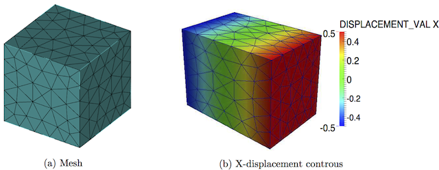
A sample mesh and corresponding x-displacement contours for a macro-strain of [1.0, 0.0, 0.0, 0.0, 0.0, 0.0] are shown in the following figure.
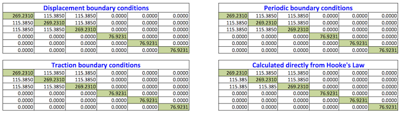
The homogenised stiffness matrices calculated using all the three types of boundary conditions are shown in the following Table. The homogenized stiffness matrices for the three type of boundary conditions are also compared with one calculated directly from the Hooke's law, which is also given in the same table. It is clear from the Table, that the homogenised stiffness matrix calculated for a homogeneous material is the same for all three types of boundary conditions and is also the same as calculated directly from the Hooke's law. In the following, the code is used for a more complex case, i.e. a unidirectional fibre reinforced composites and textile composite RVEs.
The second example consists of unidirectional fibre reinforced composites, the geometry for which is given in the following figure. Periodic mesh is created for the RVE, in which, e.g. for every nodes on the positive x-face there is a node on the negative x-face with same y and z coordinates. In this example matrix is considered as isotropic and yarn is considered as transversely isotropic materials. The following CUBIT journal file is used to create the geometry with boundary conditions and material properties. The material properties used for the matrix and fibres are given as
Matrix:
Fibres:
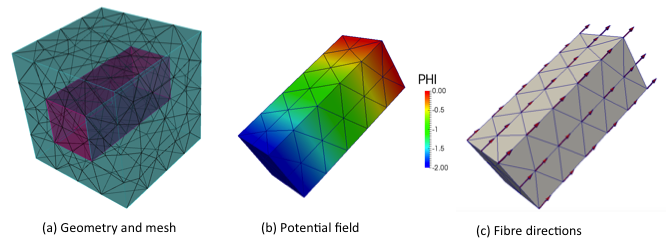
The fibre direction, required for the transversely isotropic material model is calculated by solving a potential flow problem across the fibre. The analysis procedure in this example consists of running a potential flow problem followed by actual computational homogenisation calculation. The commands used for this example is given as follows, the output of which is full homogenised stiffness matrix for linear displacement, uniform traction and periodic boundary conditions cases.
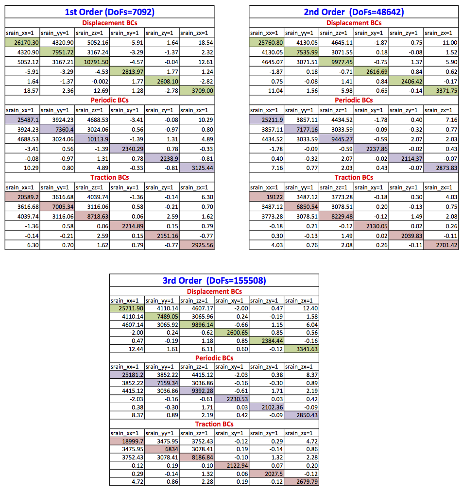
The output of the potential flow, including potential filed and calculated fibre direction are also given in the above figure. The full-homogenised stiffness matrices calculated for displacement, periodic and traction boundary conditions for 1st, 2nd and 3rd order of approximation are given in the following table.
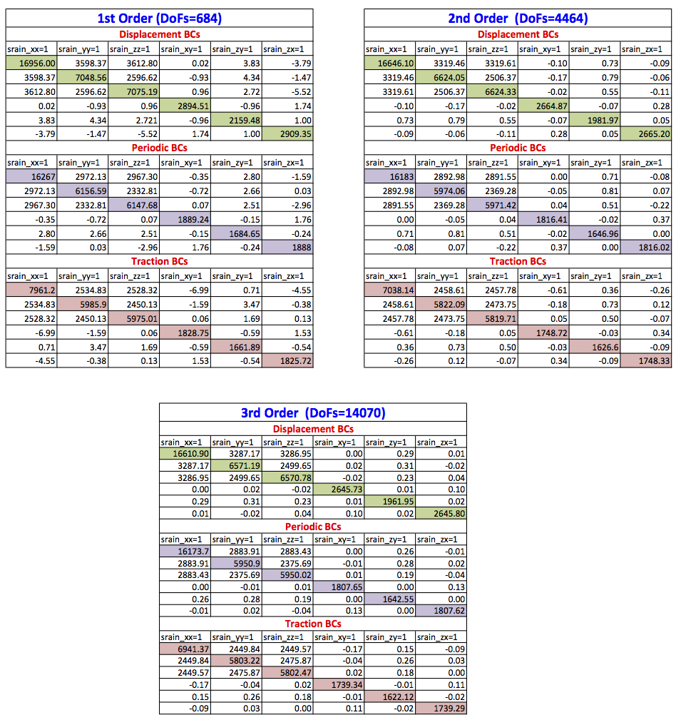
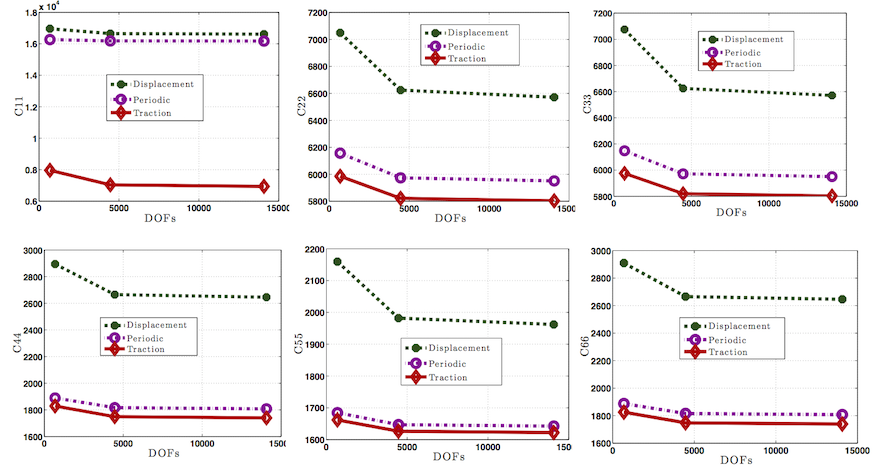
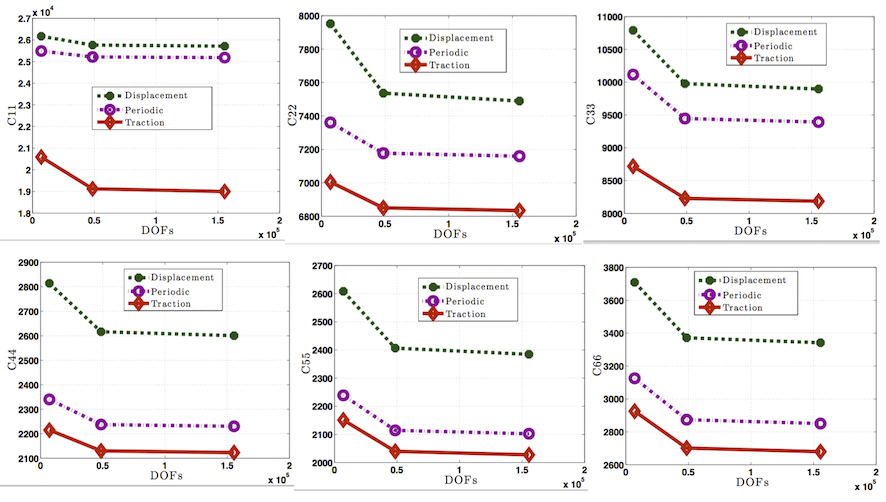
Furthermore comparison and convergence of C11, C22, C33, C44, C55 and C66 for all the three types of boundary conditions are also given in the following figure. It is clear that as expected response for the periodic boundary condition case lies between the traction and displacement boundary conditions cases. Moreover Convergence can be observed in all Cs as we increase the order of approximation from 1st to 3rd.
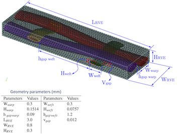
In this case a more complicated textile RVE is considered [3] consisting of matrix and textile fibres imbedded in matrix. Elliptical cross sections and cubic splines are used to model the cross-sections and paths of the fibre. Different parameters defining the RVE geometry are given in the following figure.
The CUBIT journal file required to generate the input model is given as follows (same file is used for all the three types of boundary conditions):
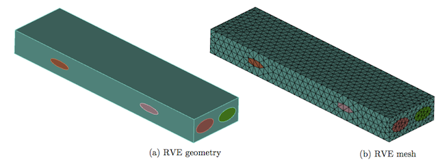
Similar to the previous unidirectional fibre reinforced composites example, matrix and fibres are considered as isotropic and transversely isotropic materials respectively with the same material properties. The finite element mesh (periodic) in this case consists of 4-node tetrahedral elements and is shown in following figure.
The commands for the calculation of e.g. the first column of the homogenised stiffness matrix for the displacement, periodic and traction boundary conditions for this example is given as
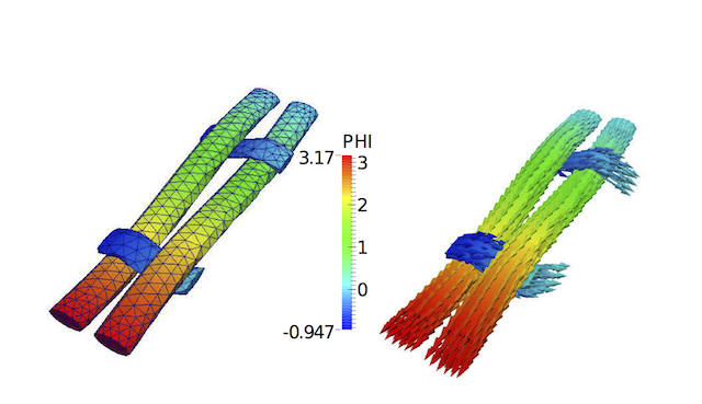
For this example, the potential field and calculated fibres directions are shown in the following figure.
Finally, the full homogenised stiffness matrices (6x6) is calculated for all the three types of boundary conditions for 1st and 2nd order of approximation and is given in the following table
Comparison of C11, C22, C33, C44, C55 and C66 for displacement, traction and periodic boundary conditions for this example are shown in the following figure. It is clear that response for the periodic boundary conditions case lies between the displacement and traction boundary conditions cases. Convergence can also be observed in C11, C22, C33, C44, C55 and C66 as we increase the order of approximation from 1st to 3rd.
Two RVE microstructures with plain weave fabric reinforcement [4, 5] and [4, 6] are selected to evaluate the applicability of computational homogenization scheme for textile composites, comparing with experimental and/or existing model results. These two models are named the Barbero model and the Scida model here after. The Barbero model is based on photomicrograph measurements of geometrical parameters and the Mori-Tanaka asymptotic homogenization method has been applied to predict the effective elastic parameters. The geometrical parameters of the Scida model were also obtained by photomicrography, and experiments were conducted to obtain the longitudinal and transversal Young’s moduli and the in-plane Poisson’s ratio. The geometry for this case with different parameters and fibres directions are shown in the following figures, in which 4a1 and 4a2 are the periodic length of warp and weft yarns, 2a3 is the waviness amplitude and ag1 and ag2 are spacing between adjacent warp and weft yarns respectively.
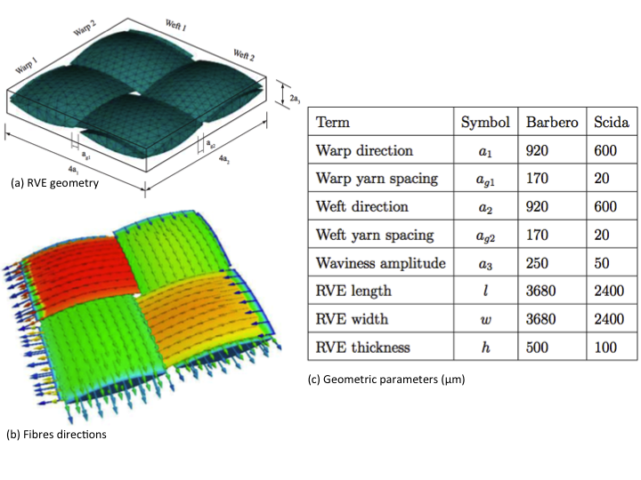
The RVE of the Barbero model has been discretized into 12148 four-node tetrahedral elements consisting of 5346 elements for the yarns and 6802 elements for the matrix, with a total of 2454 nodes, while the RVE of Scida model has been discretized into 20053 tetrahedral elements with 8101 of them for the yarns and 11952 for matrix.
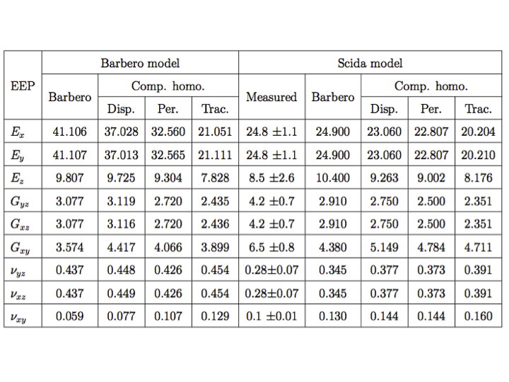
The effective engineering parameters predicted by the computational homogenization method are compared with experimental and/or numerical results. The results are listed in the following table. The reference numerical results for both models are taken from [5], where both models have been analysed using the Mori-Tanaka asymptotic homogenization method. For the Scida model, the experimental results reported are from [6]. For the computational homogenization, the results for the three boundary conditions of linear displacement, periodic, and uniform traction are given in the following table. From these results it can be seen that the model predicts moduli values that are within or very near the published standard deviation.
The CUBIT journal file used to generate the input model for Barbero RVE is given as:
The CUBIT journal file used to generate the input model for Scida RVE is given as:
Results were obtained as part of the Providing Confidence in Durable Composites (DURACOMP) project sponsored by UK Engineering and Physical Sciences Research Council (EPSRC) (Grant Ref.: EP/K026925/1).
