 |
v0.14.0 |
|
v0.14.0 |
This is an example on how to run a simulation of a gel undergoing creep and sorption due to an external load.
To examine the creep response of a gel sample, a bar section (1/8th bar) is modelled in an environment of constant relative humidity (RH) on the boundary, and with a tensile load applied in the longitudinal direction of the bar. A dirichlet BC ( \(\mu\)) is imposed on surface 4 and a Neumann symmetry condition is imposed on surface 6.
Native constitutive model is implemented after Yuhang Hu and Zhigang Suo. Viscoelasticity and poroelasticity in elastomeric gels. Acta Mechanica Solida Sinica, Vol. 25, No. 5 [32].
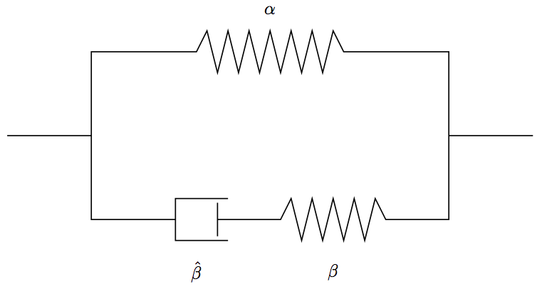
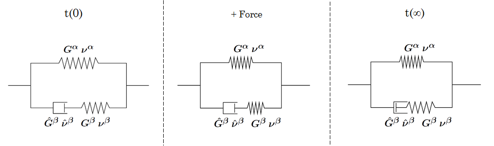
The model represents a spring, \(\alpha\), in parallel with a spring/dashpot, \(\beta\)/ \(\hat{\beta}\), in series. Initially the load is taken up by both springs, and then over time the load in spring \beta is relaxed as the dashpot, \(\hat{\beta}\), is compressed. This happens until the spring \beta is completely relaxed and the load is taken up entirely by spring \alpha. At this point the system is in equilibrium with the environment.
For more details about model implementation, equations and physical constants look here GelModule::Gel::ConstitutiveEquation
For given relative humidity chemical load is calculated form following equation,
\[ \mu = {\mu_0 + RT ln(\text{RH})) \over \text{L}} \]
where \(\mu_0\) is initial chemical potential, \(R\) is a gas constant, \(T\) is temperature, \(RH\) is relative humidity of environment (surrounding air) and \(L\) is Avogadro consistent [32].
The water vapour pressure in described in terms of relative humidity, i.e. the ratio of partial water vapour pressure to saturation pressure of the air at a given temperature. Above equation estimates the Gibb's free energy of each solvent molecule (in this case water vapour) entering the system.
Mesh is a 1/8th section of a rectangular cube, with 3 Dirichlet boundary conditions on the external faces and 3 Neumann conditions on the inner faces to impose symmetry. All dimensions are given in meters (m) and the chemical load is Gibb's free energy per solvent molecule entering the system with the units in Joules (J).
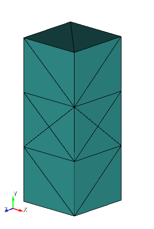
Mesh is generated in Cubit using following script,
The mesh file used in this example is located in $MODULE_DIRECTORY/meshes/creep_force.jou.
A simple section of amorphous cellulosic material is described. This material exhibits a viscoelastic response and is highly interactive with atmospheric water vapour content and makes a good case for analysis. The volume per solvent molecule (water) in it's liquid form, after chemically binding to the gel, is given by oMega in m^3. In this case the sample is initially in equilibium before the force is applied (i.e. \(\mu = \mu_0\)).
Above file can be found in $MODULE_DIRECTORY/gel_config_creep_sorption_example.in
To model the creep behaviour, a tensile force is applied in the y direction to a sample in equilibrium with it's surroundings. The application of a tensile force will encourage solvent uptake within the sample until the sample reaches equilibrium with it's environment again (i.e. increased solvent content). The load is then released, encouraging ejection of solvent from the sample until the sample once again reaches equilibrium with it's external environment.
To implement the tensile force in this manner, a load history file is used. The file includes a left hand column (time in seconds (s)) and a right hand column of load factor. In this example, a load factor of 1.0 is applied for 50000s until it is released (load factor zero) and another 50000s is allowed for the sample to recover to it's initial state.
Notes:
Running dynamic analysis out_values_1.h5m, out_values_2.h5m, ... are created for each time step. Post-processing mesh in output fails is stored in native MoAB data format using standard h5m.
VTK files can be generated using script located in users_modules/nonlinear_elasticity/do_vtk.sh. For example
To view the creep response of the material, first calculate the displacements (SPATIAL_POSISTION - coords). Plot the outside edge, furthest from the mid-point, against time. The solvent migration can also be plotted by selecting the corner that intersects all 3 inner faces (i.e. surface 1,3 and 6) and plotting against time. The results are plotted below.
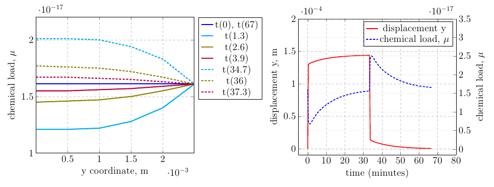
The left hand graph shows the chemical load, \(\mu\), through the sample from the top to bottom at various times given in minutes in the legend. The graph on the right gives the displacement at the top corner of the sample (left axis) vs the time in minutes. It shows the reversible creep behaviour that has been induced by the loading conditions, where immediately after the load has been released (t=33min), the sample does not go back to it's reference configuration immediately, instead taking a further 35 minutes to do so.
The right hand axis shows the chemical load at the bottom corner of the sample. Initially during the tensile loading phase, the chemical load decreases at this area of the sample, as space has been created, thus reducing the concentration. The sample responds to this by taking in more solvent in order to reach equilibrium with the environment (i.e. \( \mu \) inside the sample is equal to \( \mu \) in the environment).
After the load has been released, the extra solvent that has migrated into the sample from the environment is compressed as the sample tries to regain it's reference state, forcing the extra solvent out of the sample until equilibrium with the outside environment has been reached again.
