To examine the free-swelling response of a gel sample, a bar section is modelled in an environment of increased/decreased relative humidity (RH). A Dirichlet BC ( $\mu$) is imposed on surface 4 and a Neumann symmetry condition is imposed on surface 6. For more details how to calculate chemical load form relative humidity see Dirichelt boundary condition for chemical potential. Details about consider mechanical model can be found in Mechanical model.

Mesh

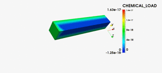
Mesh is a 1/8th section of a rectangular cube, with 3 Dirichlet boundary conditions on the external faces and 3 Neumann conditions on the inner faces to impose symmetry. All dimensions are given in metres (m) and the chemical load is Gibb's free energy per solvent molecule entering the system with the units in Joules (J).

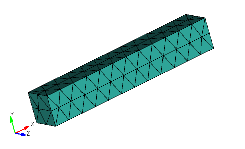
Sorption Mesh

Journal File (sorption_cube.jou)

reset
set duplicate block elements on
 
brick x 0.0025 y 0.00041 z 0.00041
 
# Set block with volume with gel material
block 1 volume all
block 1 name 'GEL'
 
# Set Dirichelt boundary condition for solvent concentration
block 2 surface 2 3 4
block 2 name 'CHEMICAL_LOAD_1'
block 2 attribute count 1
block 2 attribute index 1 6.624729054813950e-18
 
# Set solvent flux, i.e. 
block 4 surface 1 5 6
block 4 name 'FLUX_CHEMICAL_LOAD_2'
block 4 attribute count 1
block 4 attribute index 1 0
 
# Kinematic boundary condition for mechanical field
create displacement on surface 6 dof 1 fix 0
 
# Kinematic boundary condition for mechanical field
create displacement on surface 5 dof 2 fix 0
 
# Kinematic boundary condition for mechanical field
create displacement on surface 1 dof 3 fix 0
 
# Make a mesh
volume all scheme Tetmesh
volume all size auto factor 7
mesh volume all
 
# Set block 3 and set 10 node tetrahedrons in that block
block 3 tet all
block 3 element type TETRA10

Above file can be found in $GEL_MODULE_DIRECTORT/meshes/sorption_cube.jou

Material Properties

A simple section of amorphous cellulosic material is described. This material exhibits a viscoelastic response and is highly interactive with atmospheric water vapour content and makes a good case for analysis. The volume per solvent molecule (water) in it's liquid form, after binding to the gel, is given by oMega in $\text{m}^3$.

# Material parameters for Gel material model
 
# Spring Alpha
gAlpha = 6e3
vAlpha = 0.232
 
# Spring Beta
gBeta = 6e3
vBeta = 0.232
 
# Daspot
gBetaHat = 9e6
vBetaHat = 0.232
 
# Volume per solvent molecule
oMega = 2.988970058e-20
 
# Initial chemical potential
mU0 = 0
 
# Solvent transport material parameters
vIscosity = 9e6
pErmeability = 3.4e-8
 
# User can set approximation order for each blocks independently
# Set approximation order of block 1 as quadratic function.
 
[block_1]
 
oRder = 2

Above file can be found $GEL_MODULE_DIRECTORT/gel_config_creep_sorption_example.in

Chemical Load History

Changes in external environmental conditions can be implemented within the simulation using the chemical load history file. A scale factor is applied to the external BC at a given time. The input file contains the time in the left hand column and the scale factor in the right hand column. The scale factor relates the current applied chemical load to the initial applied chemical load at time zero (i.e. when the scale factor is 1.0).

To pre-determine the time of viscoelastic relaxation $(T_v)$ for each time step, the diffusivity can be calculate, entirely from the already determined material properties (section Material Properties). Taking the smallest length will be sufficient for determination in the case where adsorption is allowed on every exposed face (in this case L = 0.00041m)

\[ D = {2 \kappa \over \eta} \left( {{1-\nu^\alpha}\over{1-2\nu^\alpha}}G^\alpha + {{1-\nu^\beta}\over{1-2\nu^\beta}}G^\beta \right) \]

The time for viscoelastic relaxation, $T_v$, can then be determined

\[ T_v = {L^2 \over D} \]

The following is a chemical load history for an entire sorption cycle from 0 to 50% relative humidity and then back down to zero.

 1.000000
  1.000000000000000E+00
  1.430676558073390E+00
  1.430676558073390E+00
  1.682606194485980E+00
 1.682606194485980E+00
 1.861353116146790E+00
 1.861353116146790E+00
 2.000000000000000E+00
 2.000000000000000E+00
 2.113282752559380E+00
 2.113282752559380E+00
 2.209061955122170E+00
 2.209061955122170E+00
 2.292029674220180E+00
 2.292029674220180E+00
 2.365212388971970E+00
 2.365212388971970E+00
 2.430676558073390E+00
 2.430676558073390E+00
 2.365212388971970E+00
 2.365212388971970E+00
 2.292029674220180E+00
 2.292029674220180E+00
 2.209061955122170E+00
 2.209061955122170E+00
 2.113282752559380E+00
 2.113282752559380E+00
 2.000000000000000E+00
 2.000000000000000E+00
 1.861353116146790E+00
 1.861353116146790E+00
 1.682606194485980E+00
 1.682606194485980E+00
 1.430676558073390E+00
 1.430676558073390E+00
 1.000000000000000E+00
 1.000000000000000E+00
 0.000000000000000E+00
 0.000000000000000E+00

Above file can be found in $GEL_MODULE_DIRECTORY/my_chemical_load_history.in

Executing Problem

mpirun -np 4 ./gel_analysis -my_file sorption_cube.cub -my_gel_config \
gel_config_creep_sorption_example.in -my_chemical_load_history my_chemical_load_history.in \
-ksp_type fgmres -ksp_final_residual -ksp_monitor -ksp_converged_reason \
-pc_type lu -pc_factor_mat_solver_package mumps -my_order 3 -snes_monitor \
-ts_type beuler -ts_dt 20 -ts_final_time 70000 -my_output_prt 10 \
-snes_linesearch_type basic  -ts_monitor

Notes:

Option -my_file gives name of the mesh file
Option -my_gel_config gives the name of the material configuration file
Option -my_chemical_load_history gives the name of the chemical load history file
Option -ts_dt gives the size of each time step in seconds (s)
Option -ts_final_time gives the final time in seconds (s)
Option -my_output_prt gives the number of vtk files output (i.e. -my_output_prt 1, means each time step is processed)
Option -np gives the number of processors to run on

Results

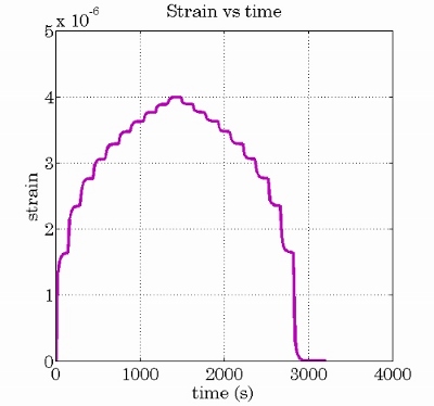
The graph below shows the overall displacement due to the chemical load entering the system. Each curve within the cycle is representative of an step change in the chemical activity on the boundary, from initial elastic response to the end of the time dependent response when all load is taken by spring \alpha.

Sorption Cycle

Deformation as result of changing environment is shown of animation below