 |
v0.14.0 |
|
v0.14.0 |
Description of density approximation from CT scan data (Usage example)
![]() This is simple example how to map density field on the finite element tetrahedral mesh from CT scan data which subsequently can be used for the bone remodelling or fracture analysis.
This is simple example how to map density field on the finite element tetrahedral mesh from CT scan data which subsequently can be used for the bone remodelling or fracture analysis.
Unlike most available material properties mapping scripts, this code not only integrates the CT scan data within finite elements but also provides approximation capabilities with many adjustable parameters. This allows to produce smooth field, neglecting the noise and inaccuracies from CT scanning.
Implementation of the following example can be found in the Bone remodeling module.
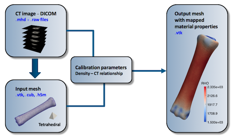
In order to conduct mapping the user has to provide CT scan data in .mhd + .raw format. It can be usually exported from the program that was used for segmentation e.g. 3D Slicer or by the conversion of standard DICOM format to Metafile by means of many available converters, like MRIConvert . Subsequently two parameters (a,b) for linear image data - density field relation has to by defined, otherwise direct CT values from the image will be mapped.
Following description and line commands are in presumption that users parent working directory is users_modules/bone_remodelling/ in build directory. All input files used in this example can be found in the example directory.
MetaImage is the text-based tagged file format for medical images included in MoFEM library. For full documentation see link . MetaIO file format (.mhd) can support a variety of objects. For density mapping simple MetaImage is used, its consists raw file that stores value of each voxel and MetaHeader file (.mhd). For example:
Above header means that we deal with 3 dimensional image that has resolution of 50 x 50 x 50 voxels (DimSize), spacing between the voxels is equal to 1 in all directions (ElementSpacing), data for each voxel is loaded from binary image.raw file (ElementDataFile) and they are float type (ElementType). Data from that file can be read easily by looping over Z, Y and X coordinates as presented in example below:
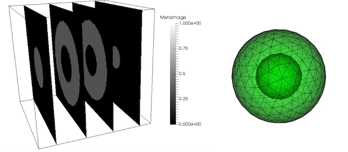
Mesh file can be created with Cubit journal file (sphere.jou),
Any other software that allows to export .vtk or .h5m mesh file can be used. User is also obligated to ensure that mesh of the mapped object is in the right position of the CT scan image. Fortunately, most of the discretisation codes do not change coordinates of segmented volumes. In this example artificial CT-data is used. All voxels inside the mesh have value equal to 1, outside 0.
Line command executing mapping should be run from users_modules/bone_remodelling/ in build directory
Notes:
\[ a\cdot CT+b=\rho \]
Execution of above command results in following outcomes:
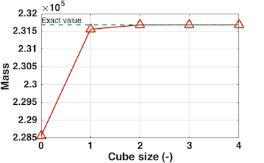
Since all voxels within mesh have value equal to 1 and default ( \(a = 1, b = 0\)) relationship was set, mapped density is 1 at any point and mass of the model should be equal to its volume.
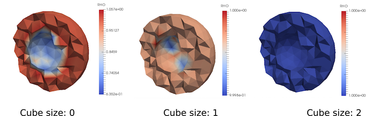
Note that for the coarse meshes (like in the example above) some of the integration points can be assigned with values of the voxels outside the volume of the CT-scanned object which can cause unwanted artifacts like presented in the figure above. To reduce that problem and achieve the exact solution, cube size parameter was adjusted.
Since high noise in CT scan data is expected, sampling volume at each integration point was implemented. Within this volume data from surounding point is collected and estimated into one value by means of 3 optional functions:
Definition of all above functions can be found in BoneRemodeling::DataFromMetaIO.
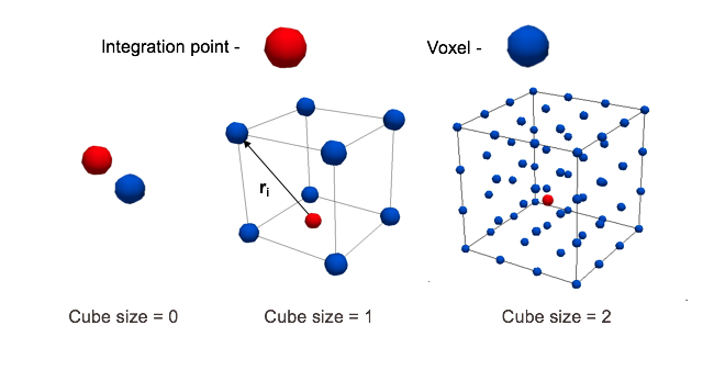
Cube dimensions are correlated with voxel size. (ElementSpacing in .mhd file) Cube size 1 means that sampling box contains 2x2x2 voxels, size 2 means 4x4x4 etc. For cube size 0, Gauss point assigns value from nearest voxel in CT image lattice, by simple rounding coordinates.
It is well know fact that raw CT scan data can be affected by so called PartialVolumeEffects. Each voxel in a CT image represents the attenuation properties of a specific material volume, if that volume is comprised of different materials (e.g bone and air) then the resulting CT value is an average of their properties. Furthermore, all object boundaries are blurred to some extent, and thus the material in any one voxel can affect CT values of surrounding voxel. To handle this problem -dist_tol parameter is introduced. Figure below presents how it works.
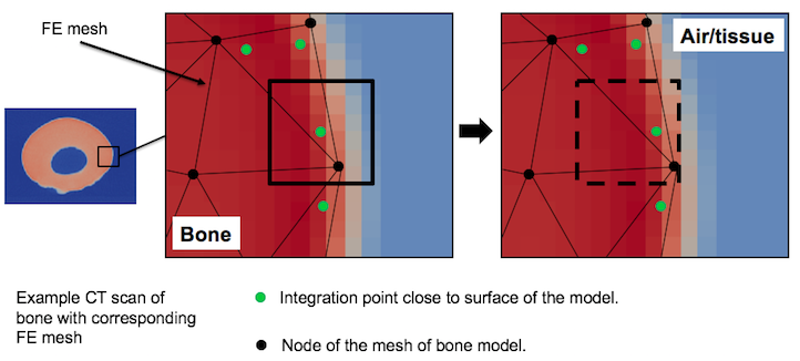
When -dist_tol parameter is used, sampling cube at every integration close to the mesh surface will be shifted by value equal to -cube_size defined. Thanks to this, voxels involved into Partial Volume Effects will not be taken into consideration during collection data for integration points. Distance of the integration points is calculated in BoneRemodeling::SurfaceKDTree class, subsequently it is used for density calculation at Gauss points in BoneRemodeling::OpCalulatefRhoAtGaussPts .
In order to produce smooth, continuous (H1 space) density field least squares approximation is proposed. The approach involves minimizing the following expression:
\[ f=\int_{V}\left(R(q,q^{\ast})\right)^{2}\,dV \]
The goal is to find values of \(q\) for the approximation which best fit the data. Least squares method finds its optimum when the sum \(f\) of squared residuals \(R\) is minimum. Herein a residual is defined as the difference between actual value of density acquired from CT scan - \(q^{\ast}\) and the approximated value \(q\), where \(\phi\) is a value of basic function at considered Gauss point:
\[ R=\phi q-q^{\ast} \]
Substituting \( R \) to the equation above results in:
\[ f=\int_{V}(\phi^{T}q^{T}-q^{\ast})(\phi q-q^{\ast})\,dV \]
In order to find minimum:
\[ \frac{\partial f}{\partial q}=\int_{V}2\phi^{T}\phi q-2\phi^{T}q^{\ast}\,dV=0 \]
This is linear system of equations:
\[ K q=\mathbf{f} \]
where:
\[ K_{e}=\int_{V_{e}}\phi\phi^{T}\,dV_{e} \qquad \mathbf{f}_{e}=\int_{V_{e}}\phi q^{\ast}\,dV_{e} \]
Above matrix \( K \) and vector \( \mathbf{f} \) are assembled in BoneRemodeling::OpCalculateLhs and BoneRemodeling::OpAssmbleRhs, respectively. Additionally, to the matrix \( K \) we introduce optional laplacian smoothing term with adjustable coefficient \( \lambda \) (-lambda parameter, can be set as 0):
\[ K_{e}=\int_{V_{e}}\phi\phi^{T}+\lambda \nabla\phi\nabla\phi^{T}\,dV_{e} \]
For full code see DensityMaps.hpp.
Sometimes it is impossible to scan long object in a CT-scanner with high resolution at once. Instead, multiple indvidual scans can be performed in order to collect all required data. Subsequently, all this data has to be merged to obtain one consistent image for the FE model or density mapping. For such purposes simple script mhd_merger.cpp was implemented. It is extremly easy to use and extendable. With a little effort CT-scan data can be resampled, cropped or even created e.g. for testing purposes. Usage example:
Execution of above command results in \en newImage.mhd file, where two images are merged into one. Voxels of the second file are shifted by vector (5,0,-2) which stands for X,Y,Z coordinates. In can be useful in case when two scans with the same resolution are not perfectly aligned.
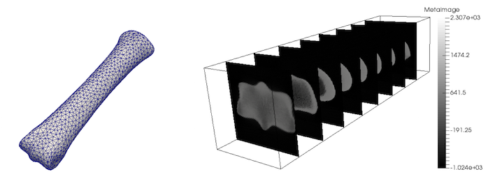
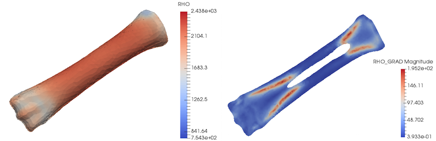
Files for the following example are: entire equine 3rd metacarpal bone CT-scan and corresponding coarse mesh. Files are also located in users_modules/bone_remodelling/examples/ directory.
Executing command:
Note that above density parameters a,b were taken from calibration phantoms which is highly recommended, since every CT scan can have a slightly different scale. Results:
Accuracy of the mapped density can be easily improved by simple increasing order of approximation:
Results of the mapping with changed order are presented below. Additionally, gradient of density field is introduced. Such plot can indicate regions with rapid changes in density which might be crucial e.g. to distinguish possible fracture locations.
Subsequently, parameter study procedure presented for the small sphere example can be followed, in order to achieve similar mass of the model as the actual object (if can be measured).
If you like contribute to this module (or MoFEM library) you are welcome. Feel free to add changes, including improving this documentation. If you like to work and modify this user module, you can fork this repository, do pull requests, see https://bitbucket.org/likask/mofem_um_bone_remodelling. Contact us cmatgu@googlegroups.com if you need any help or comments.
This user module has been co-developed by the School of Engineering and the Weipers Centre Equine Hospital, School of Veterinary Medicine at the University of Glasgow. The authors are particularly grateful to the staff of the Small Animal Hospital, where the CT scans of the equine metacarpal bone were performed. Kelvin Smith PhD Scholarship is acknowledged for providing financial support for this research.
Make a video tutorial of the presented example
Add scale parameter, in case when ct-image data and FE mesh are defined in different units (e.g. mm and m)
Input directly DICOM files (itk library)
Solving boundary and partial volume effects artifacts in a more elegant way
Add more capabilities to mhd_merger.cpp
Integrate into code (or descibe in documentation) tetrahedral meshing from .stl files by using available open source codes.
