Fracture Mechanics (Usage Examples)

Table of Contents

• Mixed mode I–III loading in three-point bending
• Graphite cylinder slice test
• Script files

Detailed step-by-step procedure for fracture simulation consisting of two numerical examples

Note

The Results in this document have been produced in the older version of the code. Command lines and input mesh files are updated to the current developement.

The following two numerical examples are given to understand the step-by-step process of simulating fracture mechanics examples within the crack propagation tools in MoFEM. For the theoretical context, the users are referred to Kaczmarczyk & Pearce [17] and Benchmarks crack propagation tests (EDF Tests) page.

How to cite us?

Mixed mode I–III loading in three-point bending

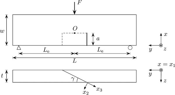
The first example presented here is the mixed mode I–III experiments of [72] on PMMA pre-notched beams loaded in a three-point-bending configuration. The experiments demonstrated that in homogeneous and linear-elastic isotropic materials the growing crack, loaded in mixed I–III mode, is observed to turn toward a pure Mode I orientation. The plates are 260mm long, 60mm deep, and 10mm thick, pre-cracked at \(45^\circ\), \(60^\circ\), and \(75^\circ\) to the front face, Figure 1. The inclination of the pre-crack results in an initially mixed mode I–III loading of the crack front.

Figure 1: Mixed mode I–III crack growth in PMMA specimen loaded in a three-point bending configuration.

Material properties used in this case are:

• Young’s modulus = 2800 MPa
• Poisson's ratio = 0.38
• Griffith energy 0.352 N/mm

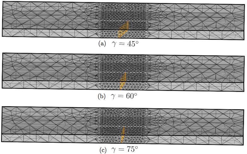
Meshes for the pre-cracked angle of \(45^\circ\), \(60^\circ\), and \(75^\circ\) are shown in Figure 2(a), 2(b) and 2(c) respectively.

Figure 2: Meshes for mixed mode I–III crack growth example.

The MOFEM input files (consisting of geometry, mesh, boundary conditions and material properties) are created with the CUBIT script file (mixed_modeI_III.jou), which will create the mixed_modeI_III.cub file in the specified directory. The same script file can be used to create input files for all the three cases by changing only the input angle.

After creating the input file, the next step is to simulate it in the MOFEM. This process is further divided into two steps. In the first step convergence study can be investigated, i.e. calculation of the Griffith forces for initial crack configuration for various h-p refinements. The following command is used to run the step-1 analysis.

mpirun -np 6 ./crack_propagation -my_file ./examples/mixed_modeI_III_45.cub -my_gc 0.352 \
-my_order 2 -my_ref 1 -my_ref_order 2 -my_propagate_crack 0  -cut_mesh 1 | tee log

where:

• -np number of processors
• -my_file mixed_modeI_III.cub mesh file
• -my_gc 0.352, material parameter, strain energy release rate
• -my_order 2, set approximation order to quadratic functions
• -my_ref 1, set mesh refinement level at crack front, 0 means no refinement
• -my_ref_order 2, set p refinement level at crack front, 0 means no refinement
• -my_propagate_crack 0 - do not run crack propagation (one elastic step only), 1 - run crack propagation

The remaining parameters will be set according to the param_file.petsc file which can be displayed on the screen with the following command:

cat param_file.petsc

Note that parameters used in the command line overwrite those in param_file.

The step-2 analysis consists of running the crack propagation, i.e.

mpirun -np 6 ./crack_propagation -my_file ./examples/mixed_modeI_III_45.cub -my_gc 0.352 \
  -nb_cut_steps 600 -nb_load_steps 3 \
  -my_order 1 -my_add_singularity 0 \
  -arc_s 1.0 -adapt_step_min_s 0.2 -adapt_step_max_s 5.0 \
  -cut_mesh 1 -ref_before_cut 1 -ref_before_tim 1 \
  -tol_cut_close 1e-1 \
  -adapt_step_its_d 8 -my_propagate_crack 1 -cut_mesh 1 | tee log

where additional parameters are,

• -arc_s 0.1 initial crack area increment, over the analysis, the step size is adapted to achieve the desired number of iterations. It controls the arc-length method.
• -adapt_step_min_s 0.01, minimal step size (crack area increment)
• -my_add_singularity 0 switch on/off singularity at the crack front
• -adapt_step_max_s 1.00, maximal step size (crack area increment)
• -adapt_step_its_d 6, desired number of iterations for load step.
• -nb_load_steps 3 number of load steps between mesh cut
• -nb_cut_steps 600 number of mesh cuts. The maximum total number of load steps before the program termination is equal to nb_cut_steps * nb_load_steps.
• -ref_before_cut 1 one level of refinment of crack surface
• -ref_before_tim 1 one level of refinment of crack front
• -tol_cut_close 1e-1 tolerance node close to crack surface

Output files from step-2 analysis are series of out_crack_surface_x.vtk and out_skin_x.h5m, where x is the load step number, ranges from 0 to the total number of load step in the simulation. File out_skin_x.h5m consists of the whole skin geometry, while out_crack_surface_x.vtk consists of crack surface only. The series of these two files can be open in ParaView for post-processing the results. The h5m files have to be converted to vtk by executing the following loop:

for f in out_skin*h5m; do mbconvert $f ${f%h5m}vtk; done

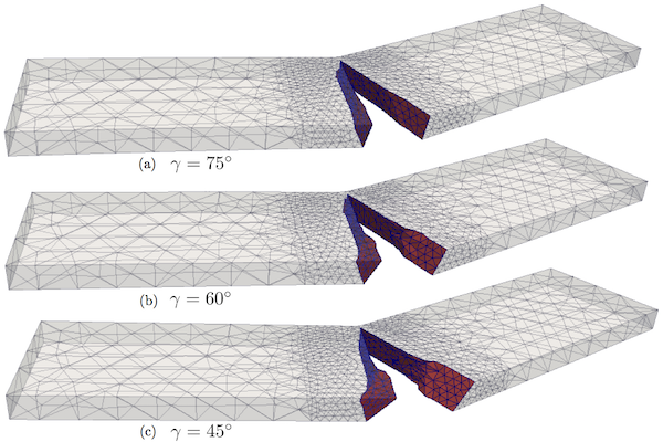
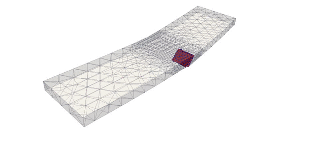
Results for the final load step with the full geometry and crack surface in case of precracked angle \(75^\circ\), \(60^\circ\), and \(45^\circ\) are shown in Figure 3(a), 3(b) and 3(c) respectively. (Note that the results presented here were produced with the old implementation)

Figure 3: Final crack surfaces for various pre-crack inclinations for mixed mode I–III crack growth example.

Furthermore, to plot the load versus displacement and elastic energy versus crack area, data need to be extracted from the output log file. This log file will be created and will consist of all output on the command line during the simulation. This can be done with the help of the commands

./scripts/plotting_data.sh 

Where log is the input and displacement_loadFactor_crackArea_energy.txt is the output file. The output of the command is in the following format, which can then be plotted accordingly, e.g. in MATLAB or Excel.

-1               0               0               0               0
 0         32.4848           2.608      2.3747e+02  4.23602026e+01
 1         32.4936           2.608      2.3749e+02  4.23716368e+01
 2         32.5057           2.608      2.3750e+02  4.23873954e+01
 3         32.5087           2.609      2.3753e+02  4.24076315e+01
 4         32.5163            2.61      2.3754e+02  4.24337750e+01

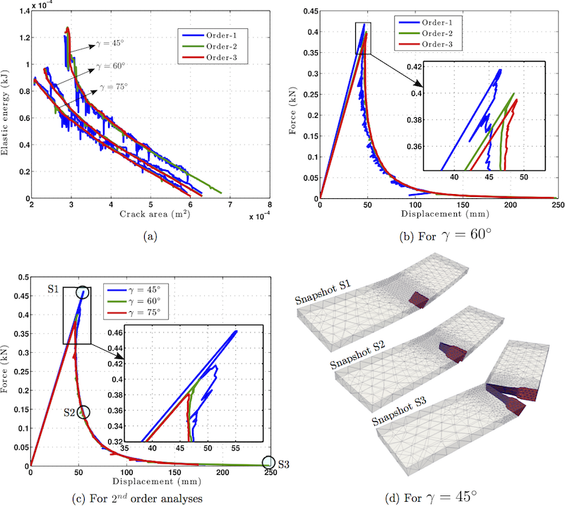
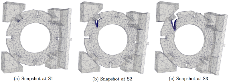
Where colums from left to right are: step number, displacement, load factor, crack area and energy, respectively. This problem is analysed with 1st, 2nd and 3rd order of approximation. Results for elastic energy (column-4) versus crack area (column-2) is shown in Figure 4(a), consisting of results for nine simulations. It is clear from Figure 4(a) that for a given cracked surface area, the precracked sample with smaller angles (e.g. \(\gamma = 45^\circ\)) possesses more elastic energy. Moreover, results are fluctuating for 1st order analysis and increasing the order of approximation leads to smoother results. Convergence analysis for load versus generalised displacement (explained in documentation page Benchmarks crack propagation tests) with respect to order of approximation for a pre-cracked angle of \(\gamma = 60^\circ\) is shown in Figure 4(b). The ultimate load for 1st-order, 2nd-order and 3rd-order order analyses are 0.42 kN, 0.4 kN and 0.395 kN respectively. Comparison of load versus generalised displacement plots for different pre-cracked angles for 2nd-order analyses are shown in Figure 4(c). The ultimate load for \(\gamma = 45^\circ\), \(\gamma = 60^\circ\) and \(\gamma = 75^\circ\) are 0.46 kN, 0.4 kN and 0.38 kN respectively with decreasing trend. Snapshots of evolving crack for 2nd-order analyses and \(\gamma = 45^\circ\) case, for points S1, S2 and S2, shown in Figure 4(c), are shown in Figure 4(d).

Figure 4: Elastic energy versus crack area and force versus displacement plots for 1st-order, 2nd-order and 3rd-order of approximation and various pre-crack inclinations for mixed mode I–III crack growth example.

An animation of full fracturing process for \(\gamma = 45^\circ\) is shown in the following.

Graphite cylinder slice test

This second numerical example considers a slice of a graphite cylindrical brick, placed in a loading rig and loaded as shown in Figure 5.

Figure 5: Experimental loading frame for graphite cylinder slice test. All dimensions in mm.

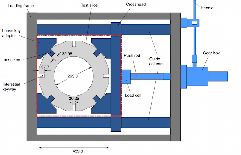
The red box indicates the part modelled in the numerical analysis. The loose key adaptors on the left are fully fixed along their left hand side. The numerical load is applied to the mid-point of the crosshead beam.

Material properties used in this case are

• Young’s modulus = 10,900 MPa
• Poisson's ratio = 0.2
• Griffith energy 0.23 N/mm

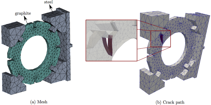
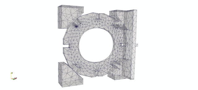
The input file for the analysis consisting of geometry, mesh, boundary conditions and material properties are created using CUBIT. The mesh is shown in Figure 6(a).

Figure 6: Geometry and crack path for graphite cylinder slice test.

The script file, brick_slice_test.jou is used to create the input file brick_slice_test.cub in the user specified directory.

Similar to the previous example, simulation consists of the following two steps:

mpirun -np 6 ./crack_propagation -my_file ./examples/brick_slice_test_paper.cub \
-my_gc 0.23e-4 -my_add_singularity 0 \
-nb_cut_steps 600 -nb_load_steps 3 \
-my_order 1 -my_ref_order 2 -ref_before_tim 1 \
-arc_s 1 -adapt_step_min_s 0.1 -adapt_step_max_s 20 \
-adapt_step_its_d 8 -my_propagate_crack 1 -cut_mesh 1 \
-edges_block_set 4 -vertex_block_set 5 | tee log

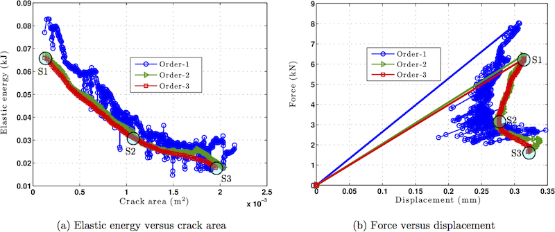
It should be noted that within the above-mentioned commands, material properties are multiplied with 1e-4 (This is only to help in Newton-Raphson's method convergence). The numerically predicted crack path is shown in Figure 6(b). It can be seen that the crack propagates from the keyway corner with a curved trajectory to the free surface of the inner bore. This problem is solved with 1st, 2nd and 3rd order of approximation. The elastic energy versus the crack area and the force versus generalised displacement plots are shown in Figures 7(a) and 7(b) respectively. The experimental ultimate load was 6.2 kN. The numerical ultimate loads were 7.79 kN, 6.42 kN, 6.25 kN for the 1st-order, 2nd-order, 3rd-order analyses respectively as shown in Figure 7(b). (Note that the results presented here were produced with the old implementation)

Figure 7: Energy versus crack area and load versus displacement plots for graphite cylinder slice test

Snapshots of the brick slice at three points S1, S2 and S3, shown in Figure 7 are shown in Figure 8(a), 8(b) and 8(c) respectively. In order to generate deformation in Paraview paraview_deform_macro.py can be added and used as a Macro.

Figure 8: Snap shots for points S1, S2 and S3 shown in Figure 7 for graphite cylinder slice test.

An animation of full fracturing process is also shown in the following.

Script files

Script file for mixed mode I–III loading in three-point bending mixed_modeI_III.jou

Script file for graphite cylinder slice test brick_slice_test.jou

Acknowledgements

This work was supported by the EDF Energy Nuclear Generation Ltd. The views expressed in this document are those of the authors and not necessarily those of the EDF Energy Nuclear Generation Ltd.

Analyses were undertaken using the EPSRC funded ARCHIE- WeSt High Performance Computer (www.archie-west.ac.uk).