 |
v0.14.0 |
|
v0.14.0 |
The present tutorial is aimed to introduce elementary concepts of the Finite Element Method (FEM) with hierarchical shape functions and their implementation in MoFEM.
The reader is assumed to be familiar with the FEM approach to solve Partial Differential Equations (PDEs). Here, differences between the node oriented (that most readers are familiar with) and hierarchical shape functions is described. Aspects of MoFEM implementation of this approach will be described for the user to understand the FEM implementation within the present framework. These concepts are presented as briefly as possible with sole aim to clarify their implementation within MoFEM.
Advantages of the Hierarchical shape functions are not going to be described in the present tutorial. The key points for choosing MoFEM implementation of the FEM method with Hierarchical basis functions instead of the node oriented approach are presented in this section to clearly set the motivation behind this particular choice. Choosing Hierarchical basis functions over node oriented basis is that it results to:
In the FEM, the unknown field \(u({\mathbf {x}}) \) is approximated as
\[ \begin{equation} u({\mathbf {x}}) \approx u^h({\mathbf {x}}) = \sum_{i=1}^{n} N_i u_i \label{eq:Approx} \end{equation} \]
where \({\mathbf{ x}}\) denotes the coordinate vector, \(u\) is the function to be approximated, \(u^h\) is the approximating function and \(N_i\) are the shape functions associated with the \(n\) number of degrees of freedom \(u_i\) of a particular choice.
Node oriented shape functions are always associated with the degrees of freedom corresponding to a node. Node oriented shape functions are presented for a 1D element in Figure 1 a, b and c for first, second and third order, respectively. For simplicity we will be restricted to 1D element for the moment. Each degree of freedom is associated with a node and has a physical meaning. In the case of p- and hp- adaptivity, where the order of approximation is chosen to increase at certain regions of the domain, this kind of shape functions increase the complexity of implementation since new meshes with extra nodes must be generated.

These complexities can be resolved by using hierarchical shape functions. Examples of hierarchical shape functions in a 1D element are presented in Figure 2 a, b and c for first, second and third order, respectively. By inspection of Figure 2 b and c it can be seen that no extra nodes are added for functions of order higher than the first one. This feature makes the p- and hp- adaptivity implementation much easier since no extra nodes are needed to be introduced into the mesh.
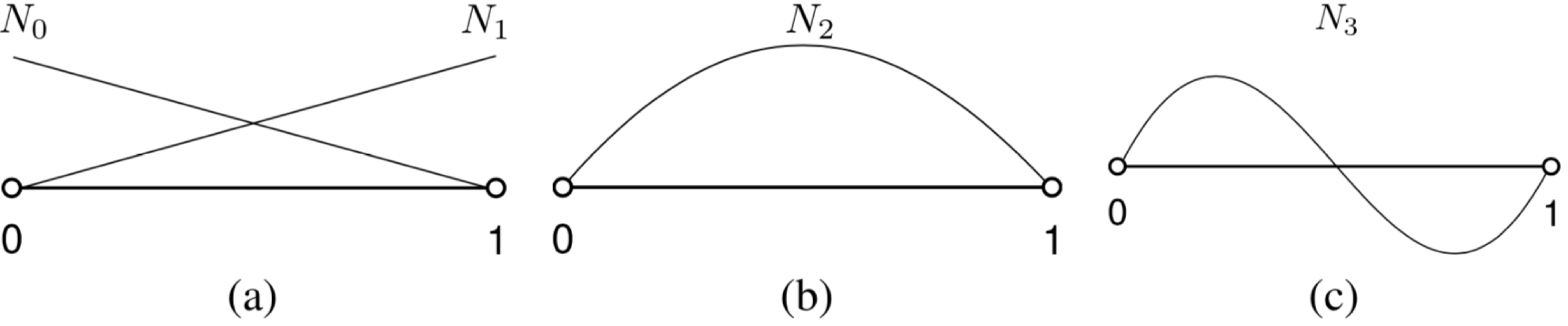
Furthermore, all but the first order functions are unique (i.e. there is only one function of each order) and identically zero at the element nodes. For the first order there are two functions, one for each node. Partition of unity is therefore preserved at the nodes but not necessarily in-between. Hence, for order of choice \(p\) the number of degrees of freedom is going to \(p + 1\).
For the 1D case, only the first two degrees of freedom ( \(u_i\)) presented in \( \eqref {eq:Approx}\) are associated with the nodes. The rest of the degrees of freedom are free of any node notion and there is no particular need to be linked to a physical value. These degrees of freedom are purely mathematical.
From now on nodes will be referred as vertices and the entity generated by the 1D space that connects the two vertices will be referred as edge.
A practical way of assembling the degrees of freedom associated to a 1D element can be done by separation of the degrees of freedom associated with vertices (first order) to those with edges (higher orders). Therefore, the elemental degrees of freedom \({\mathbf{ n}^e}\) of a 1D element can be presented as
\[ \begin{equation} {\mathbf {u}^e} = \left[ \begin{array}{c c} {\mathbf { n}^e} &{\mathbf { e}^e} \end{array} \right] \label{eq:ElementDOF1D} \end{equation} \]
where \({\mathbf { n}^e}\) and \({\mathbf { e}^e}\) are sub-vectors containing degrees of freedom associated with vertices and the edge, respectively. According to \(\eqref {eq:Approx} \), \({\mathbf { n}^e}\) will always be consisted of two degrees of freedom as presented below
\[ \begin{equation} {\mathbf { n}^e} = \left[ \begin{array}{cc} u_0 & u_1 \\ \end{array} \right] \label{eq:VertexDOF1} \end{equation} \]
However, the length of \({\mathbf { e}^e}\) depends on the order of approximation chosen. For \(p = 1 \) , \({\mathbf { e}^e}\) will have no members. For \(p = 3 \) the vector will have two members and it will have the form
\[ \begin{equation} {\mathbf { e}^e} = \left[ \begin{array}{cc} u_2 & u_3 \\ \end{array} \right] \label{eq:VertexDOF2} \end{equation} \]
Similar separation can be performed with the corresponding shape functions. Usefulness of the separation will become apparent later and it is intrinsic to the implementations that will be presented in this tutorial.
These concepts can be extended to 2D and 3D elements. In 1D the two entities that were presented were vertex and edge. The extra entities that emerge in the 2D and 3D domains are faces and volumes, respectively.
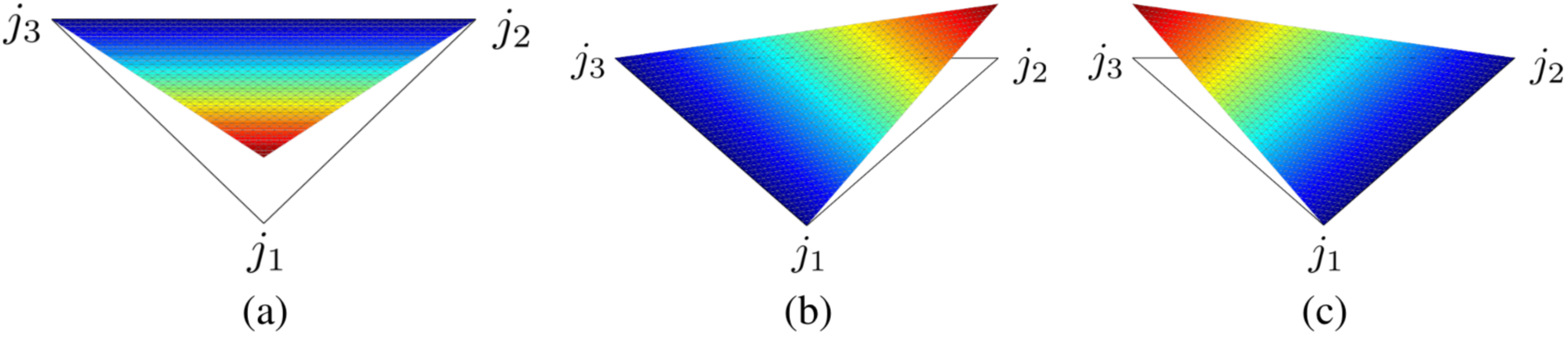
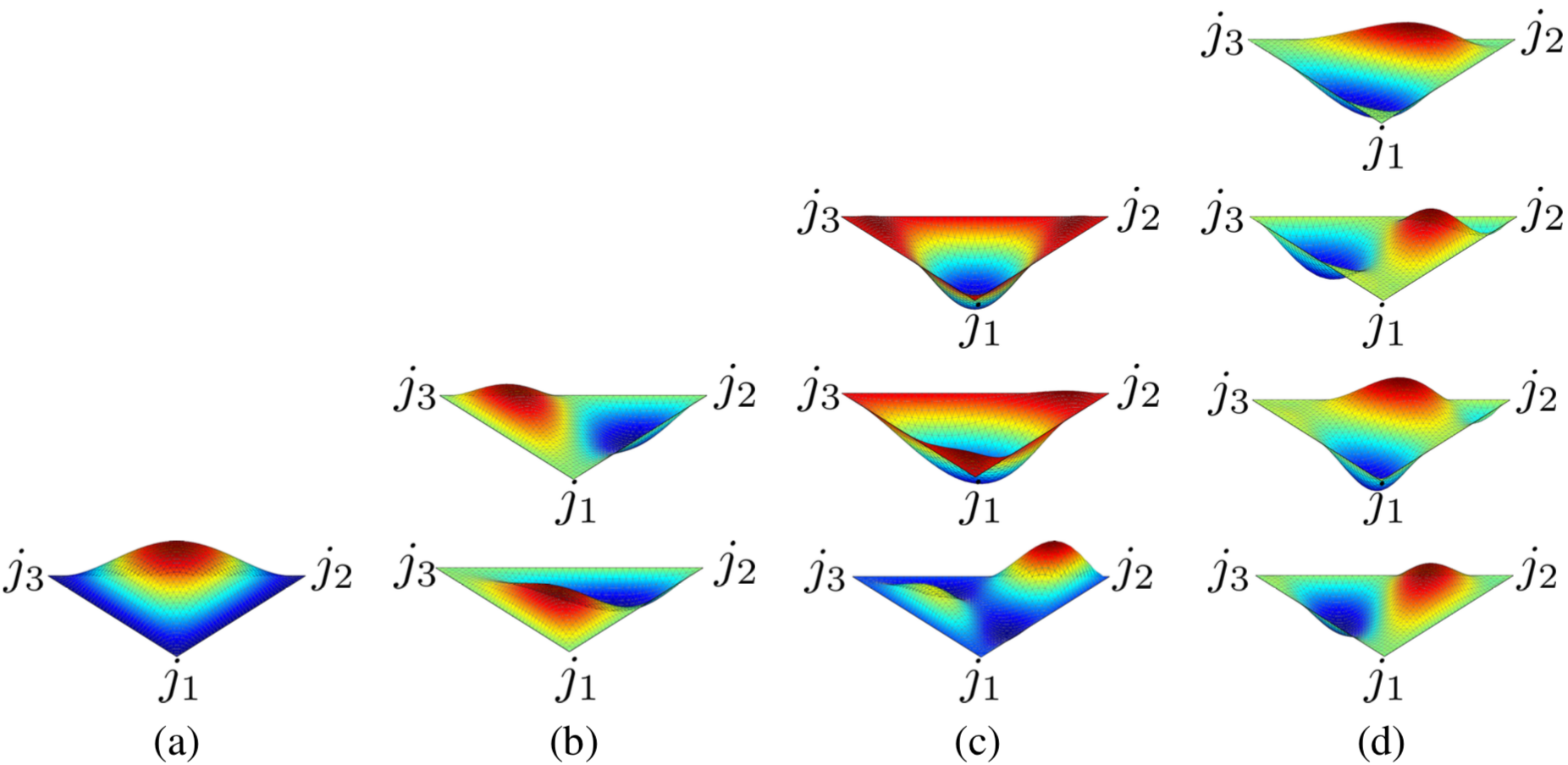
Shape functions that can be found implemented in MoFEM now are associated with vertices, edges, triangular faces and tetrahedral volumes. The shape functions for edges that are part of triangular faces and the shape functions of triangular faces are presented in Figure 4 and Figure 5, respectively. The values of the shape functions along the 2D space of a face can be thought as the varying height or depth of the nonlinear surfaces from the planar triangular face. When the curved surface is below or above the planar face, the shape function takes negative or positive values, respectively. Vertex shape functions are equal to unity at their associated vertices and identically zero along the opposite edge and one the other two vertices. The edge functions are always identically zero at all vertices and along all edges except for the associated edge. The face functions are generally non zero on the face area but are always zero on vertices and along edges.
The volume shape functions are not presented in this tutorial due to the high complexity of their presentation in a 2D fashion. However, the reader can imagine the volume shape functions as smooth grey colour changes in 3D space. When a location is white or black coloured then the shape function takes its minimum or maximum values. Furthermore, volume shape functions are identically zero on vertices and along edges and faces of the associated tetrahedron.

Now the concept of decomposition of elemental degrees of freedom described by the equation \(\eqref {eq:ElementDOF1D}\) can be taken further from a 1D element to the 3D tetrahedron element. In fact, it will be evident that this decomposition applies to any type of 3D element under consideration. Now the vector of the degrees of freedom \({\mathbf {u}^e}\) of one element is
\[ \begin{equation} {\mathbf { u}^e} = \left[ \begin{array}{cccc} {\mathbf { n}^e} & {\mathbf { e}^e} & {\mathbf { f}^e} & {\mathbf { v}^e} \end{array} \right] \label{eq:ElementDOF3D} \end{equation} \]
where \({\mathbf { f}^e}\) and \({\mathbf { v}^e}\) are the sub-vectors containing the degrees of freedom associated with the face and volume shape functions, respectively. Therefore, the number of degrees of freedom for each sub-vector associated with an entity is equal to the number of shape functions associated with that particular entity. For instance, when the shape functions presented in Figure 4 and Figure 5 are used, \({\mathbf { e}^e}\) and \({\mathbf { f}^e}\) contain nine and ten degrees of freedom, respectively.
Similarly, the vector of shape functions of an element can be decomposed into four sub vectors
\[ \begin{equation} {\mathbf {N}^e} = \left[ \begin{array}{cccc} {\mathbf {N}^e_{\textrm {ver}}} & {\mathbf {N}^e_{\textrm {edge}}} & {\mathbf {N}^e_{\textrm {face}}} & {\mathbf {N}^e_{\textrm {vol}}} \\ \end{array} \right] \label{eq:ElementShape3D} \end{equation} \]
where \({\mathbf {N}^e}\) is the vector of the element's shape function and \({\mathbf {N}^e_{\textrm {ver}}}\), \({\mathbf {N}^e_{\textrm {edge}}}\), \({\mathbf {N}^e_{\textrm {face}}}\) and \({\mathbf {N}^e_{\textrm {vol}}}\) are the sub-vectors of the shape functions associated with vertices, edges, faces and volume respectively.
Here it should be mentioned that the choice of the entities and their associated degrees of freedom and shape functions under consideration for solutions of boundary value problems are dictated by the particular choice of the shape function space and the order of approximation. The case where all entities' shape functions are taken into account is for the H1 space for \(p\geq4\). Spaces that can be used in MoFEM are also L2, H-curl and H-Div that are sub-spaces of H1. For the sake of simplicity, this tutorial will proceed assuming an H1 space with \(p\geq4\) in order to have all entities degrees of freedom and shape functions in the examples. Discussion on the particular choice of shape function space will be presented in another tutorial.
One of the most common proccesses encompassed within the Finite Element Method is the evaluation of the stiffness matrix. The evaluation of the element stiffness matrix is going to be presented by making use of the decomposition of degrees of freedom and shape functions presented in \(\eqref {eq:ElementDOF3D}\) and \(\eqref {eq:ElementShape3D}\).
The stiffness matrix of a volume element is evaluated as the integral of
\[ \begin{equation} {\mathbf {\textrm K}^e} = \int_{\Omega^e}({\mathbf {\nabla^{T}N}^e})^{\textrm T} {\mathbf {\nabla^{\textrm T} N}^e} {\textrm d\Omega^e} \label{eq:StiffnessIntegral} \end{equation} \]
where \({\mathbf {\textrm K}^e}\) is the element stiffness matrix, \(\Omega^e\) is the element domain and \({\mathbf {\rm \nabla^{\textrm T}}}\) is the vector form of the first order gradient operator taken as
\[ \begin{equation} {\mathbf {\rm \nabla}}^{\rm T} = \left[ \begin{array}{c} \dfrac{\partial}{\partial x}\\ \dfrac{\partial}{\partial y}\\ \dfrac{\partial}{\partial z}\\ \end{array} \right] \label{eq:Nabla} \end{equation} \]
hence the product \({\mathbf {\nabla^{\textrm T} N}^e}\) can be evaluated as
\[ \begin{equation} \begin{split} {\mathbf {\nabla^{\textrm T} N}^e} = \left[ \begin{array}{c} \dfrac{\partial}{\partial x}\\ \dfrac{\partial}{\partial y}\\ \dfrac{\partial}{\partial z}\\ \end{array} \right] \left[ \begin{array}{cccc} {\mathbf {N}^e_{\textrm ver}} & {\mathbf {N}^e_{\textrm edge}} & {\mathbf {N}^e_{\textrm face}} & {\mathbf {N}^e_{\textrm vol}} \end{array} \right] = \left[ \begin{array}{cccc} \dfrac{\partial {\mathbf {N}^e_{\textrm ver}} }{\partial x} & \dfrac{\partial {\mathbf {N}^e_{\textrm edge}} }{\partial x} & \dfrac{\partial {\mathbf {N}^e_{\textrm face}} }{\partial x} & \dfrac{\partial {\mathbf {N}^e_{\textrm vol}} }{\partial x} \\ \dfrac{\partial {\mathbf {N}^e_{\textrm ver}} }{\partial y} & \dfrac{\partial {\mathbf {N}^e_{\textrm edge}} }{\partial y} & \dfrac{\partial {\mathbf {N}^e_{\textrm face}} }{\partial y} & \dfrac{\partial {\mathbf {N}^e_{\textrm vol}} }{\partial y}\\ \dfrac{\partial {\mathbf {N}^e_{\textrm ver}} }{\partial z} & \dfrac{\partial {\mathbf {N}^e_{\textrm edge}} }{\partial z} & \dfrac{\partial {\mathbf {N}^e_{\textrm face}} }{\partial z} & \dfrac{\partial {\mathbf {N}^e_{\textrm vol}} }{\partial z} \\ \end{array} \right] = \left[ \begin{array}{cccc} {\mathbf {\nabla^{\textrm T} N}^e_{\textrm ver}} & {\mathbf {\nabla^{\textrm T} N}^e_{\textrm edge}} & {\mathbf {\nabla^{\textrm T} N}^e_{\textrm face}} & {\mathbf {\nabla^{\textrm T} N}^e_{\textrm vol}} \end{array} \right] \end{split} \label{eq:NablaShape1} \end{equation} \]
therefore the product \(({\mathbf {\nabla^{\textrm T} N}^e})^{\textrm T} {\mathbf {\nabla^{\textrm T} N}^e}\) is evaluated as
\[ \begin{equation} \begin{split} ({\mathbf {\nabla^{\textrm T} N}^e})^{\textrm T} {\mathbf {\nabla^{\textrm T} N}^e} = \left[ \begin{array}{c} ({\mathbf {\nabla^{\textrm T} N}^e_{\textrm {ver}}})^{\rm T}\\ ({\mathbf {\nabla^{\textrm T} N}^e_{\textrm {edge}}})^{\rm T}\\ ({\mathbf {\nabla^{\textrm T} N}^e_{\textrm {face}}})^{\rm T}\\ ({\mathbf {\nabla^{\textrm T} N}^e_{\textrm {vol}}})^{\rm T} \end{array} \right] \left[ \begin{array}{cccc} {\mathbf {\nabla^{\textrm T} N}^e_{\textrm {ver}}} & {\mathbf {\nabla^{\textrm T} N}^e_{\textrm {edge}}} & {\mathbf {\nabla^{\textrm T} N}^e_{\textrm {face}}} & {\mathbf {\nabla^{\textrm T} N}^e_{\textrm {vol}}} \end{array} \right] =\\ \\ = \left[ \begin{array}{cccc} ({\mathbf {\nabla^{\textrm T} N}^e_{\textrm {ver}}})^{\rm T} {\mathbf {\nabla^{\textrm T} N}^e_{\textrm {ver}}} & ({\mathbf {\nabla^{\textrm T} N}^e_{\textrm {ver}}})^{\rm T} {\mathbf {\nabla^{\textrm T} N}^e_{\textrm {edge}}} & ({\mathbf {\nabla^{\textrm T} N}^e_{\textrm {ver}}})^{\rm T} {\mathbf {\nabla^{\textrm T} N}^e_{\textrm {face}}} & ({\mathbf {\nabla^{\textrm T} N}^e_{\textrm {ver}}})^{\rm T} {\mathbf {\nabla^{\textrm T} N}^e_{\textrm {vol}}}\\ ({\mathbf {\nabla^{\textrm T} N}^e_{\textrm {edge}}})^{\rm T} {\mathbf {\nabla^{\textrm T} N}^e_{\textrm {ver}}} & ({\mathbf {\nabla^{\textrm T} N}^e_{\textrm {edge}}})^{\rm T} {\mathbf {\nabla^{\textrm T} N}^e_{\textrm {edge}}} & ({\mathbf {\nabla^{\textrm T} N}^e_{\textrm {edge}}})^{\rm T} {\mathbf {\nabla^{\textrm T} N}^e_{\textrm {face}}} & ({\mathbf {\nabla^{\textrm T} N}^e_{\textrm {edge}}})^{\rm T} {\mathbf {\nabla^{\textrm T} N}^e_{\textrm {vol}}} \\ ({\mathbf {\nabla^{\textrm T} N}^e_{\textrm {face}}})^{\rm T} {\mathbf {\nabla^{\textrm T} N}^e_{\textrm {ver}}}& ({\mathbf {\nabla^{\textrm T} N}^e_{\textrm {face}}})^{\rm T} {\mathbf {\nabla^{\textrm T} N}^e_{\textrm {edge}}}& ({\mathbf {\nabla^{\textrm T} N}^e_{\textrm {face}}})^{\rm T} {\mathbf {\nabla^{\textrm T} N}^e_{\textrm {face}}}& ({\mathbf {\nabla^{\textrm T} N}^e_{\textrm {face}}})^{\rm T} {\mathbf {\nabla^{\textrm T} N}^e_{\textrm {vol}}} \\ ({\mathbf {\nabla^{\textrm T} N}^e_{\textrm {vol}}})^{\rm T} {\mathbf {\nabla^{\textrm T} N}^e_{\textrm {ver}}}& ({\mathbf {\nabla^{\textrm T} N}^e_{\textrm {vol}}})^{\rm T} {\mathbf {\nabla^{\textrm T} N}^e_{\textrm {edge}}}& ({\mathbf {\nabla^{\textrm T} N}^e_{\textrm {vol}}})^{\rm T} {\mathbf {\nabla^{\textrm T} N}^e_{\textrm {face}}}& ({\mathbf {\nabla^{\textrm T} N}^e_{\textrm {vol}}})^{\rm T} {\mathbf {\nabla^{\textrm T} N}^e_{\textrm {vol}}} \\ \end{array} \right] \end{split} \label{eq:FullStiffness} \end{equation} \]
In dynamic analyses, mass matrix is an extra component to solve the discrete problem. The stiffness matrix of a volume element is evaluated as the integral of
\[ \begin{equation} {\mathbf {\textrm M}^e} = \int_{\Omega^e}({\mathbf {N}^e})^{\textrm T} {\mathbf {N}^e} {\textrm d\Omega^e} \label{eq:MassMatrixIntegral} \end{equation} \]
where \({\mathbf {\textrm M}^e}\) is the element mass matrix. Similar to the element stiffness matrix, the matrix quantity in the integrals is evaluated similar to \(\eqref {eq:FullStiffness}\) as
\[ \begin{equation} \begin{split} ({\mathbf {N}^e})^{\textrm T} {\mathbf {N}^e} = \left[ \begin{array}{c} ({\mathbf {N}^e_{\textrm {ver}}})^{\rm T}\\ ({\mathbf {N}^e_{\textrm {edge}}})^{\rm T}\\ ({\mathbf {N}^e_{\textrm {face}}})^{\rm T}\\ ({\mathbf {N}^e_{\textrm {vol}}})^{\rm T} \end{array} \right] \left[ \begin{array}{cccc} {\mathbf {N}^e_{\textrm {ver}}} & {\mathbf {N}^e_{\textrm {edge}}} & {\mathbf { N}^e_{\textrm {face}}} & {\mathbf {N}^e_{\textrm {vol}}} \end{array} \right] = \\ \left[ \begin{array}{cccc} ({\mathbf {N}^e_{\textrm {ver}}})^{\rm T} {\mathbf {N}^e_{\textrm {ver}}} & ({\mathbf {N}^e_{\textrm {ver}}})^{\rm T} {\mathbf {N}^e_{\textrm {edge}}} & ({\mathbf {N}^e_{\textrm {ver}}})^{\rm T} {\mathbf {N}^e_{\textrm {face}}} & ({\mathbf {N}^e_{\textrm {ver}}})^{\rm T} {\mathbf {N}^e_{\textrm {vol}}}\\ ({\mathbf {N}^e_{\textrm {edge}}})^{\rm T} {\mathbf {N}^e_{\textrm {ver}}} & ({\mathbf {N}^e_{\textrm {edge}}})^{\rm T} {\mathbf {N}^e_{\textrm {edge}}} & ({\mathbf {N}^e_{\textrm {edge}}})^{\rm T} {\mathbf {N}^e_{\textrm {face}}} & ({\mathbf {N}^e_{\textrm {edge}}})^{\rm T} {\mathbf {N}^e_{\textrm {vol}}} \\ ({\mathbf {N}^e_{\textrm {face}}})^{\rm T} {\mathbf {N}^e_{\textrm {ver}}}& ({\mathbf {N}^e_{\textrm {face}}})^{\rm T} {\mathbf {N}^e_{\textrm {edge}}}& ({\mathbf {N}^e_{\textrm {face}}})^{\rm T} {\mathbf {N}^e_{\textrm {face}}}& ({\mathbf {N}^e_{\textrm {face}}})^{\rm T} {\mathbf {N}^e_{\textrm {vol}}} \\ ({\mathbf {N}^e_{\textrm {vol}}})^{\rm T} {\mathbf {N}^e_{\textrm {ver}}}& ({\mathbf {N}^e_{\textrm {vol}}})^{\rm T} {\mathbf {N}^e_{\textrm {edge}}}& ({\mathbf {N}^e_{\textrm {vol}}})^{\rm T} {\mathbf {N}^e_{\textrm {face}}}& ({\mathbf {N}^e_{\textrm {vol}}})^{\rm T} {\mathbf {N}^e_{\textrm {vol}}} \\ \end{array} \right] \end{split} \label{eq:FullMass} \end{equation} \]
To assemble the global stiffness matrix to solve the discretised problem, three nested loops are performed. The out most loop operates over the finite elements, the second loop operated over the element entities and the innermost loop operates over the element gauss points.
In a typical implementation, the user can access base functions on the finite element for each sub-entity of finite element. For example, the quadrilateral is made from four nodes, four edges and one quadrilateral face. The tetrahedron is constructed from four nodes, six edges, four faces and one tetrahedron volume. Developer can access base functions on those entities by structure MoFEM::EntitiesFieldData::EntData. This structure carries basic on information entity, like approximation order, orientation (sense), number of DOFs, and base functions, etc.. It is accessed from Users Data Operator explained in other tutorials.
In particular, base functions are accessed on entity by MoFEM::EntitiesFieldData::EntData::getN and derivatives by MoFEM::EntitiesFieldData::EntData::getDiffN. Here we explain the structure of matrices returned by those two functions. Note that those functions are overloaded and have many variants for developer convenience, and derivatives of them for H-div and H-curl spaces.
Assembling contribution from finite element, for each entity on finite element MoFEM calls the developer overridden implementation of User Data Operator, i.e. method MoFEM::DataOperator::doWork. You can see how such operator is implemented for example in COR-6: Solid elasticity.
The goal of the loop over element entities is to assemble the element stiffness matrix presented in \(\eqref {eq:FullStiffness}\). The set of information associated to each entity is row_data and col_data which are instances of MoFEM::EntitiesFieldData::EntData and passed as argument in MoFEM::DataOperator::doWork. In col_data the matrix \({\mathbf {\nabla^{\textrm T} N}^e_{\textrm {ent}}}\) presented in \(\eqref {eq:FullStiffness}\) is stored. In \(row\_data\), a series of matrices \(({\mathbf {\nabla^{\textrm T} N}^e_{\textrm {ent}}})^{\rm T}\) is stored presented in \(\eqref {eq:FullStiffness}\), where \({\mathbf {N}}^e_{\textrm {ent}}\) is the shape function of a given entity. Each entity (ent), has two matrices \(({\mathbf {\nabla^{\textrm T} N}^e_{\textrm {ent}}})^{\rm T}\) and \({\mathbf {\nabla^{\textrm T} N}^e_{\textrm {ent}}}\) as well as shape functions corresponding to the entities degrees of freedom. These matrices are stored as rows in matrices, where each row corresponds to a gauss point as presented in \(\eqref {eq:NablaShape1}\)
\[ \newcommand{\myarray}[1]{{\left\downarrow\vphantom{#1}\right.{#1}}} \newcommand{\myarraysecond}[1]{{\overset{\xrightarrow[\hphantom{#1}]{\text{$n$ degrees of freedom of element entity}}}{#1}}} \begin{equation} \text{element $m$ gauss points}\myarray{ \begin{array}{c} \\ {\rm {gg}}_1 \\ \\ {\rm {gg}}_2 \\ \\ {\rm {gg}}_3 \\ \\ \vdots \\ {\rm {gg}}_m \end{array} } \myarraysecond{ \left[ \begin{array}{ccccc} {\overbrace{\begin{array}{c c c} \dfrac{\partial {\mathbf {N}^e_{\textrm 1}} }{\partial x} & \dfrac{\partial {\mathbf {N}^e_{\textrm 1}} }{\partial y} & \dfrac{\partial {\mathbf {N}^e_{\textrm 1}} }{\partial z} \end{array} }^{\textrm{1st Element DoF} } } &\dots & \dfrac{\partial {\mathbf {N}^e_{ n}} }{\partial x} & \dfrac{\partial {\mathbf {N}^e_{ n}} }{\partial y} & \dfrac{\partial {\mathbf {N}^e_{ n}} }{\partial z} \\ {\begin{array}{c c c} \dfrac{\partial {\mathbf {N}^e_{\textrm 1}} }{\partial x} & \dfrac{\partial {\mathbf {N}^e_{\textrm 1}} }{\partial y} & \dfrac{\partial {\mathbf {N}^e_{\textrm 1}} }{\partial z}\end{array}} & \dots & \dfrac{\partial {\mathbf {N}^e_{ n}} }{\partial x} & \dfrac{\partial {\mathbf {N}^e_{ n}} }{\partial y} & \dfrac{\partial {\mathbf {N}^e_{n}} }{\partial z} \\ {\begin{array}{c c c}\dfrac{\partial {\mathbf {N}^e_{\textrm 1}} }{\partial x} & \dfrac{\partial {\mathbf {N}^e_{\textrm 1}} }{\partial y} & \dfrac{\partial {\mathbf {N}^e_{\textrm 1}} }{\partial z}\end{array}} & \dots & \dfrac{\partial {\mathbf {N}^e_{ n}} }{\partial x} & \dfrac{\partial {\mathbf {N}^e_{ n}} }{\partial y} & \dfrac{\partial {\mathbf {N}^e_{ n}} }{\partial z} \\ {\begin{array}{c c c c c}\vdots\,\, & & \vdots & & \,\, \vdots \end{array}} & \ddots & \vdots & \vdots &\vdots \\ {\begin{array}{c c c}\dfrac{\partial {\mathbf {N}^e_{\textrm 1}} }{\partial x} & \dfrac{\partial {\mathbf {N}^e_{\textrm 1}} }{\partial y} & \dfrac{\partial {\mathbf {N}^e_{\textrm 1}} }{\partial z}\end{array}} & \dots & \dfrac{\partial {\mathbf {N}^e_{ n}} }{\partial x} & \dfrac{\partial {\mathbf {N}^e_{ n}} }{\partial y} & \dfrac{\partial {\mathbf {N}^e_{ n}} }{\partial z} \end{array} \right] } \hspace{2.cm} \label{eq:NablaShape2} \end{equation} \]
For the same gauss point \({\rm {gg}}_m\), row data from matrices \(\eqref {eq:NablaShape2}\) and \(\eqref {eq:ShapeGG}\) is retrieved and a loop is performed to evaluate all multiplication of degree of freedom combination.
Similarly, the mass matrix presented in \(\eqref {eq:FullMass}\) is evaluated performing the loop over the element entities and gauss points where the shape functions are stored to a matrix data structure as presented below
\[ \newcommand{\myarray}[1]{{\left\downarrow\vphantom{#1}\right.{#1}}} \newcommand{\myarraysecond}[1]{{\overset{\xrightarrow[\hphantom{#1}]{\text{$n$ degrees of freedom of element entity}}}{#1}}} \begin{equation} \text{element $m$ gauss points}\myarray{ \begin{array}{c} {\rm {gg}}_1 \\ {\rm {gg}}_2 \\ {\rm {gg}}_3 \\ \vdots \\ {\rm {gg}}_m \end{array} } \myarraysecond{ \left[ \begin{array}{ccccccc} \mathbf {N}^e_{\textrm 1} & {\mathbf {N}^e_{\textrm 2}} & {\mathbf {N}^e_{\textrm 3}} & \dots & {\mathbf {N}^e_{n-2}} & {\mathbf {N}^e_{ n-1}} & {\mathbf {N}^e_{n}} \\ {\mathbf {N}^e_{\textrm 1}} & {\mathbf {N}^e_{\textrm 2}} & {\mathbf {N}^e_{\textrm 3}} & \dots & {\mathbf {N}^e_{n-2}} & {\mathbf{N}^e_{n-1}} & {\mathbf {N}^e_{n}} \\ {\mathbf {N}^e_{\textrm 1}} & {\mathbf {N}^e_{\textrm 2}} & {\mathbf {N}^e_{\textrm 3}} & \dots & {\mathbf {N}^e_{n-2}} & {\mathbf {N}^e_{n-1}} & {\mathbf {N}^e_{n}}\\ \vdots & \vdots & \vdots & \ddots & \vdots & \vdots &\vdots \\ {\mathbf {N}^e_{\textrm 1}} & {\mathbf {N}^e_{\textrm 2}} & {\mathbf {N}^e_{\textrm 3}} & \dots & {\mathbf {N}^e_{n-2}} & {\mathbf {N}^e_{n-1}} & {\mathbf {N}^e_{n}} \end{array} \right] } \hspace{2.5cm} \label{eq:ShapeGG} \end{equation} \]
Note that there is no notion of the shape of the element since matrices are integrated and assembled entity-by-entity, which in finite element. This implementation approach is completely general. To evaluate the element stiffness matrix one need to list entities, and on them gauss points, degrees of freedom, shape functions and their gradients and perform the aforementioned loop.
