 |
v0.14.0 |
|
v0.14.0 |
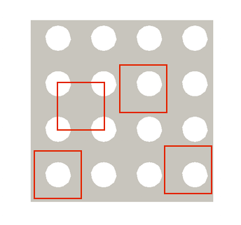
In this document we will study a material example which contains periodically distributed voids. In the case of a material with a periodic structure, one can choose the smallest possible unit cell such that in repeating this cell in the array, the material microstructure is reproduced without additional gaps. Note, it is not unique how the unit cell is constructed, i.e. the void can be placed perfectly in the centre or frame of the unit cell or it can be arbitrarily shifted leaving the void off centre. In the figure below the red frames represent some subjectively selected unit cells. If periodic boundary conditions are applied to these unit cell, homogenised overall stress and a material tangent matrix are invariant to the selection of the unit cell frame and results are objective.
![]()
For periodic boundary conditions, displacements on the opposite sides of the representative volume element (RVE) are constrained as follows
\[ \mathbf{u}_+-\mathbf{u}_-={\boldsymbol \varepsilon}^M(\mathbf{x}_+-\mathbf{x}_-) \]
where \(+\) and \(-\), denote opposite sides of the RVE, \(\mathbf{u}\) is the displacement vector and \({\boldsymbol \varepsilon}^M\) represents macro-strain. Here for simplicity we restrict ourselves to small strain. Such constrains enforce that
\[ {\boldsymbol \varepsilon}^M = \frac{1}{V} \int_\Omega {\boldsymbol \varepsilon} \textrm{d}\Omega = \frac{1}{V} \int_\Gamma \textrm{sym}[\mathbf{n}\otimes\mathbf{u}] \textrm{d}\Gamma. \]
Moreover, periodic boundary conditions satisfy the Hill-Mandel condition meaning that the energy expressed in terms macro quantities is equal to energy expressed in terms micro quantities
\[ {\boldsymbol \varepsilon}^M:{\boldsymbol \sigma}^M = \frac{1}{V} \int_\Omega {\boldsymbol \varepsilon}:{\boldsymbol \sigma} \textrm{d}\Omega = \frac{1}{V} \int_\Gamma \mathbf{u}\cdot\mathbf{n}{\boldsymbol \sigma} \textrm{d}\Gamma, \]
where \(\mathbf{n}\) is the unit normal to the surface. All above equations and boundary integrals are true assuming that the equilibrium equation
\[ \textrm{div}[{\boldsymbol \sigma}] = \mathbf{0} \]
is satisfied for all points within the RVE. See [37] for details. In this paper the equilibrium equation is satisfied in the weak sense.
Applying periodic constraints to a discreet problem requires that surface meshes on opposite sides must have matching geometry, i.e. nodal positions and topology. In general for simple geometries such meshes can be generated easily, however for more complex microstructures (for example in crystallography) generation of periodic meshes is non-trivial. Nitsche's method enables the user to apply periodic constraints on non-periodic meshes, however in this document we focus on problem formulation, where technicalities related to numerical integration on non-matching meshes are not discussed.
In the first part we will derive the unified Nitsche's method with generic multipoint constrains. Next a special case of periodic constraints is shown. After that, implementation aspects of the method are briefly discussed. finally at the end a simple numerical example is presented.
If you would like to add a more sophisticated example to this documentation, please contact us at cmatgu@googlegroups.com. We will help you to install MoFEM and guide you on how to use it. Implementation of Nitsche's method is general (see Nitsche Method), and could be extended to other problems, for example, contact at a cohesive interface, general contact problems, sliding boundary conditions etc. If you are interested in solving kinds of problems, we can help you with the implementation.
In the course of learning Nitsche's method we typically follow two papers, see [27] and [36], this is an excellent starting point from which one can discover a vast pool literature on the subject. In the following document and implementation (see Nitsche Method), general symmetric and non-symmetric variants of the method are presented.
Dirichlet constraints need to be satisfied a priori by proper choice of approximation basis. This can be done easily when point constrains are applied; by erasing rows and columns in the stiffness matrix. In the case of multi-point constraints such as those found when using periodic boundary conditions, a Lagrange multiplier method can be used (see this link) or projection operators can be constructed (see [37]) to enforce constraints.
The Nitsche's method on the other hand enforces kinematic constrains in the weak sense by replacing Dirichlet constrains with additional Neumann terms in bilinear form. This method allows for greater flexibility which extends far beyond the simple application presented here. In this paper we focus on enforcing periodic constraints of an arbitrary shaped convex RVE.
In the following section for convenience we using Voigt (vector-matrix) notation, where
\[ \boldsymbol\varepsilon = \{ \varepsilon_{xx},\, \varepsilon_{yy},\, \varepsilon_{zz},\, 2\varepsilon_{xy},\, 2\varepsilon_{yz},\, 2\varepsilon_{xz} \}. \]
The considered problem is restricted to a RVE, therefore body forces or any boundary conditions are neglected, only kinematic constraints enforced on the RVE boundary are factored in. In this section we do not intended to give a formal and precise prerequisite, defining the considered function spaces and detailed proofs, our focus is on the application and simplicity of the document.
We consider an elastic body in the reference domain \(\Omega\) with a sufficiently smooth boundary \(\Gamma\). For simplicity, we restrict formulation to linear elasticity, however implementation in MoFEM is general and extends to non-linear cases. The considered weak problem takes the well known form
\[ \begin{equation} a(\mathbf{u},\mathbf{v}) - \int_\Gamma {\boldsymbol\sigma}^\textrm{T}(\mathbf{u})\mathbf{n}^\textrm{T}\mathbf{v} \textrm{d}\Gamma = 0, \quad \forall \mathbf{v} \end{equation} \]
where \(\mathbf{n}\) is a normal on the surface \(\Gamma\), \(\boldsymbol\sigma\) is a stress calculated from the hyperelastic physical equation, \(\mathbf{u}\) and \(\mathbf{v}\) are displacement and test functions respectively. We will now consider a case in which both displacements and test functions belong to the standard Lagrange finite element space such that weak form can be expressed by a system of algebraic equations. Note that the Lagrange finite element approximation space is a dense and finite subspace of \(H^1(\Omega)\).
The traction force on the RVE boundary \(\Gamma\) in the spirit of Nitsche's method is given by
\[ \mathbf{t}(\mathbf{u}) = \mathbf{n}{\boldsymbol\sigma} = -\frac{1}{\gamma} \mathcal{R}(\mathcal{C}\mathbf{u}-\mathbf{g}-\gamma\mathcal{C}\mathbf{t}(\mathbf{u})) \quad\textrm{on}\,\Gamma \]
where \(\gamma := \gamma(x) > 0\) is some bounded (continuity condition) positive function defined on the RVE boundary, \(\mathcal{C}\) is a linear constraint operator and \(\mathbf{g}\) is a constraint function. Since we restrict ourselves to Lagrange finite element spaces constraints can be written as an algebraic condition. Taking this into account the operator \(\mathcal{R}\) is defined by
\[ \mathcal{R} = \mathcal{C}^\textrm{T}(\mathcal{C}\mathcal{C}^\textrm{T})^{-1}, \]
and the constraint projection operator is given by
\[ \mathcal{P} = \mathcal{R}\mathcal{C}. \]
Note that the projection operator has the well-known property, \(\mathcal{P} = \mathcal{P}\mathcal{P}\). The constraint operator \(\mathcal{C}\), gives a well posed problem if constraints are not too restrictive and matrix \(\mathcal{C}\) is full rank. See [4] for details on how algebraic projection operators are constructed. Here operator \(\mathcal{C}\) and dependent operators are acting on approximation functions rather than on the function value at a specific point in space. Here we are simply considering the finite element approximation, thus \(\mathcal{C}\) can be seen as a matrix which operates on multiple degrees of freedom potentially on multiple nodes (entities). Now let \(\phi\) be some fixed real value parameter and noting that
\[ \mathbf{v} = \mathcal{R}(\mathcal{C}\mathbf{v}-\phi\gamma\mathcal{C}\mathbf{t}(\mathbf{v})) +\phi\gamma\mathcal{P}\mathbf{t}(\mathbf{v}) + \mathcal{Q}\mathbf{v} \]
where \(\mathcal{Q}=\mathcal{I}-\mathcal{P}\). To show that the above relationship is true, see that \(\mathcal{R}\mathcal{C}=\mathcal{P}\) and \(\mathcal{P}+\mathcal{Q}=\mathcal{I}\). After [27] and [36] is proposed, \(\gamma\) turns out to be a positive constant function on the RVE face.
\[ \gamma(x) = \gamma_0. \]
Having definition of tractions and test functions, the weak problem takes on the form of a generalised Nitsche's method.
\[ \begin{split} a(\mathbf{u},\mathbf{v}) - \sum_E \int_\Gamma \phi \gamma_0 \mathbf{t}^{\textrm{T}}(\mathbf{u}) \mathcal{P}\mathbf{t}(\mathbf{v}) \textrm{d}\Gamma + \sum_E \int_\Gamma \frac{1}{\gamma_0} \mathcal{R}(\mathcal{C}\mathbf{v}-\phi \gamma_0\mathcal{C}\mathbf{t}(\mathbf{v})) \textrm{d}\Gamma = 0 \quad \forall \mathbf{v} \end{split} \]
\[ \begin{split} a(\mathbf{u},\mathbf{v}) - \sum_E \int_\Gamma \phi \gamma_0 \mathbf{t}^{\textrm{T}}(\mathbf{u}) \mathcal{P}\mathbf{t}(\mathbf{v}) \textrm{d}\Gamma + \sum_E \int_\Gamma \frac{1}{\gamma_0} \left\{ \mathbf{u}-\gamma_0\mathbf{t}(\mathbf{u})) \right\}^\textrm{T} \mathcal{P} (\mathbf{v}-\phi \gamma_0\mathbf{t}(\mathbf{v})) \textrm{d}\Gamma = \sum_E \int_\Gamma \frac{1}{\gamma_0} \mathbf{g}^\textrm{T}\mathcal{R}^\textrm{T} (\mathbf{v}-\phi \gamma_0\mathbf{t}(\mathbf{v})) \textrm{d}\Gamma \quad \forall \mathbf{v} \end{split} \]
which some simplifications this lead to
\[ \begin{split} a(\mathbf{u},\mathbf{v}) - \sum_E \int_\Gamma \left\{ \mathbf{t}^\textrm{T}(\mathbf{u})\mathcal{P}\mathbf{v} + \phi\mathbf{u}^\textrm{T}\mathcal{P}\mathbf{t}(\mathbf{v}) \right\} \textrm{d}\Gamma + \sum_E \int_\Gamma \frac{1}{\gamma_0} \mathbf{u}^\textrm{T}\mathcal{P}\mathbf{v} \textrm{d}\Gamma = \sum_E \int_\Gamma \frac{1}{\gamma_0} \mathbf{g}^\textrm{T}\mathcal{R}^\textrm{T} \mathbf{v} \textrm{d}\Gamma - \phi \int_\Gamma \mathbf{t}^\textrm{T}(\mathbf{v}) \mathcal{R}\mathbf{g} \textrm{d}\Gamma \quad \forall \mathbf{v} \end{split} \]
Since we restrict ourselves to standard finite element approximation, the above equation can be expressed in in algebraic form,
\[ \left[ \mathbf{A} - (\mathbf{A}_\sigma+\phi\mathbf{A}^\textrm{T}_\sigma) + \frac{1}{\gamma_0}\mathbf{A}_{\gamma_0} \right] \mathbf{q} = \frac{1}{\gamma_0}\mathbf{f}_{\gamma_0}-\phi\mathbf{f}_\phi \]
where \(\mathbf{q}\) is a vector of unknown degrees of freedom, in addition we define the auxiliary matrix
\[ \mathbf{A}_\phi = (\mathbf{A}_\sigma+\phi\mathbf{A}^\textrm{T}_\sigma) \]
and finally we get
\[ \left[ \mathbf{A} - \mathbf{A}_\phi + \frac{1}{\gamma_0}\mathbf{A}_{\gamma_0} \right] \mathbf{q} = \frac{1}{\gamma_0}\mathbf{f}_{\gamma_0}-\phi\mathbf{f}_\phi \]
where matrices are defined as follows
\[ \mathbf{A} = \int_\Omega \mathbf{B}^\textrm{T}\mathbf{D}\mathbf{B} \textrm{d}\Omega, \quad \mathbf{A}_\sigma = \sum_E \int_\Gamma \mathbf{N}^\textrm{T} \mathcal{P} \mathbf{n}\mathbf{D}\mathbf{B} \textrm{d}\Gamma, \quad \mathbf{A}_{\gamma_0} = \sum_E \int_\Gamma \mathbf{N}^\textrm{T} \mathcal{P} \mathbf{N} \textrm{d}\Gamma, \]
where \(\mathbf{N}\) is a matrix of shape functions, \(\mathbf{B}\) is the standard differential operator, such that \(\boldsymbol\varepsilon(\mathbf{u})=\mathbf{B}\mathbf{u}\), \(\mathbf{D}\) is the material stiffness matrix and \(\boldsymbol\sigma(\mathbf{u})=\mathbf{D}\mathbf{B}\mathbf{u}\) where
\[ \mathbf{n}= \left[ \begin{array}{cccccc} n_1 & 0 & 0 & n_2 & 0 & n_3 \\ 0 & n_2 & 0 & n_1 & n_3 & 0 \\ 0 & 0 & n_3 & 0 & n_2 & n_3 \end{array} \right], \]
In which \(n_1\), \(n_2\) and \(n_3\) are components of the unit normal vector on the body surface. The right hand side vectors are defined as follows
\[ \mathbf{f}_{\gamma_0} = \sum_E \int_\Gamma \mathbf{N}^\textrm{T}\mathcal{R}\mathbf{g} \quad \mathbf{f}_\phi = \phi \sum_E \int_\Gamma \mathbf{B}^\textrm{T}\mathbf{D}\mathbf{n}^\textrm{T} \mathcal{R}\mathbf{g} \textrm{d}\Gamma. \]
After [27] introduction of the numerical parameter \(\phi\), allows for us to include some variants acting on the symmetry / skew-symmetry / non-symmetry of the discrete formulation.
Suppose that the exact solution of a continuous problem with constraints ( \(\mathcal{C}\mathbf{u} - \mathbf{g} = \mathbf{0}\)), is exactly interpolated on the finite element approximation space. We show that Nitsche's method is consistent with such an exact solution. Taking the weak equation
\[ \begin{split} a(\mathbf{u},\mathbf{v}) - \sum_E \int_\Gamma \mathbf{t}^{\textrm{T}}(\mathbf{u}) \phi\gamma\mathcal{P}\mathbf{t}(\mathbf{v}) \textrm{d}\Gamma + \sum_E \int_\Gamma \frac{1}{\gamma_0} \left\{ \mathcal{R}(\mathcal{C}\mathbf{u}-\mathbf{g}-\gamma\mathcal{C}\mathbf{t}(\mathbf{u})) \right\}^\textrm{T} \mathcal{R}(\mathcal{C}\mathbf{v}-\phi\gamma\mathcal{C}\mathbf{t}(\mathbf{v})) \textrm{d}\Gamma = 0 \end{split} \]
and substituting the tractions approximation
\[ \mathbf{t}(\mathbf{u}) = -\frac{1}{\gamma} \mathcal{R}(\mathcal{C}\mathbf{u}-\mathbf{g}-\gamma\mathcal{C}\mathbf{t}(\mathbf{u})), \]
as a result of simple algebraic manipulations, the standard weak from is recovered
\[ a(\mathbf{u},\mathbf{v}) - \int_\Gamma {\boldsymbol\sigma}^\textrm{T}(\mathbf{u})\mathbf{N}^\textrm{T}\mathbf{v} \textrm{d} \Gamma = 0. \]
This shows the solution of Nitsche's method is a solution of original problem with constraints. In other words, as long as the problem is well-posed, solution of Nitsche's method converges to the original problem with the given constraints. Note that penalty method solution is not consistent, in a sense that the solution of the original problem with constraints is not a solution when penalty terms enforce constraints.
In using the classical penalty method, to verify correctness of the results one needs to show that results converge for both increasing mesh density (approximation order) and for \(\gamma_0 \to 0\). Since Nitsche's method is consistent, it is only necessary to demonstrate solution convergence when we refining mesh or increasing approximation order. Here \(\gamma_0\) is understood as the stabilisation parameter which controls the convergence rate. However, since we work with finite precision arithmetics, \(\gamma_0\) cannot be too small to have well a conditioned matrix.
If a problem is considered 'well posed' it means that a solution exist, this is a unique characteristic which depends continuously on the boundary conditions. In the example below we will detail a coercive problem, this implies that the stiffness matrix is positively defined. Note that this does not imply symmetry of the operator on right hand side. Our focus here is on simplicity of the argumentation rather than on strict formal mathematical proof.
After [27] we use following property (*)
\[ \int_\Gamma \mathbf{t}^\textrm{T}(\mathbf{v}) \mathcal{P} \mathbf{t}(\mathbf{v}) \textrm{d}\Gamma \leq C_I a(\mathbf{v},\mathbf{v}) \]
and using that finite element approximation is applied, i.e. \(\mathbf{v} = \mathbf{N}\mathbf{q}\), we get
\[ \int_\Gamma \mathbf{t}^\textrm{T}(\mathbf{v}) \mathcal{P} \mathbf{t}(\mathbf{v}) \textrm{d}\Gamma \leq C_I \mathbf{q}^\textrm{T} \mathbf{A} \mathbf{q} \]
Moreover, we assume that the initial problem without constraints is well posed, i.e. rigid body motion is restricted, below we can see that matrix \(\mathbf{A}\) is positively defined
\[ \mathbf{q}^\textrm{T} \mathbf{A} \mathbf{q} \geq C \mathbf{q}^\textrm{T}\mathbf{q} \]
In addition, using properties of the projection matrix \(\mathcal{P}\), it is noted that matrix \(\mathbf{A}_{\gamma_0}\) is semi-positively defined.
To show that the problem is coercive, the following methodology from [27] and [36], for given equality
\[ \mathbf{q}^\textrm{T} (\mathbf{A}-\mathbf{A}_\phi+\frac{1}{\gamma_0}\mathbf{A}_{\gamma_0}) \mathbf{q} = \mathbf{q}^\textrm{T} \mathbf{A} \mathbf{q} - \int_\Gamma \left\{ \mathbf{t}^\textrm{T}(\mathbf{v})\mathcal{P}\mathbf{v} + \phi\mathbf{v}^\textrm{T}\mathcal{P}\mathbf{t}(\mathbf{v}) \right\} \textrm{d}\Gamma + \gamma_0 \mathbf{q}^\textrm{T} \mathbf{A}_{\gamma_0} \mathbf{q} \]
and using property (*) and applying Young's inequality in above we get
\[ \mathbf{q}^\textrm{T} (\mathbf{A}-\mathbf{A}_\phi+\frac{1}{\gamma_0}\mathbf{A}_{\gamma_0}) \mathbf{q} \geq \mathbf{q}^\textrm{T} \left\{ \mathbf{A} - C_I\epsilon\frac{1+\phi}{2} \mathbf{A} - \frac{(1+\phi)}{2\epsilon} \mathbf{A}_{\gamma_0} + \gamma_0\mathbf{A}_{\gamma_0} \right\} \mathbf{q}. \]
\[ \mathbf{q}^\textrm{T} (\mathbf{A}-\mathbf{A}_\phi+\frac{1}{\gamma_0}\mathbf{A}_{\gamma_0}) \mathbf{q} \geq \mathbf{q}^\textrm{T} \left\{ \left(1-C_I\epsilon\frac{1+\phi}{2}\right)\mathbf{A} + \left(\frac{1}{\gamma_0}-\frac{(1+\phi)}{2\epsilon}\right)\mathbf{A}_{\gamma_0} \right\} \mathbf{q}. \]
where \(\epsilon>0\). Having the above inequality at hand we can consider following variants,
We note that matrix \(\mathbf{A}\) doesn't necessary has to restrict translation or rotation, if matrix \(\mathbf{A}_{\gamma_0}\) constrains translation or rotation, respectively. In other words, the sum of matrices \(\mathbf{A}\) and \(\mathbf{A}_{\gamma_0}\) has to be a full rank matrix.
In this section we consider periodic boundary conditions which are applied by Nitsche's method by specifying appropriate constraint matrices and vectors. Let constraint matrix be given by
\[ \mathcal{C} = [\mathbf{I},-\mathbf{I}], \]
where \(\mathbf{I}\) is unit matrix (3x3). The auxiliary matrix is given by
\[ \mathcal{R} = \frac{1}{2} \left\{ \begin{array}{c} \mathbf{I}\\ -\mathbf{I} \end{array} \right\} \]
and the projection matrix has the form
\[ \mathcal{P} = \frac{1}{2} \left[ \begin{array}{cc} \mathbf{I} & -\mathbf{I}\\ -\mathbf{I} & \mathbf{I} \end{array} \right] \]
In addition, we define matrices
\[ \mathbf{E}(\mathbf{x}) = \frac{1}{2} \left[ \begin{array}{cccccc} 2x & 0 & 0 & y & 0 & z \\ 0 & 2y & 0 & x & z & 0 \\ 0 & 0 & 2z & z & 0 & x \end{array} \right] \]
and get the constraint vector as follows
\[ \mathbf{g} = \mathcal{P}\mathbf{D}{\boldsymbol\varepsilon}^M = (\mathbf{E}_{+}-\mathbf{E}_{-}){\boldsymbol\varepsilon^M}. \]
where \({\boldsymbol\varepsilon}^M\) is the macroscopic stress vector in Voigt notation. Finally, the constraint matrix has the form,
\[ \mathcal{C}\left\{ \mathbf{q}_+, \mathbf{q}_- \right\} = \mathbf{g} \]
where \(+\) and \(-\) indicate points the on boundary of the RVE on opposite sides. We assume an arbitrary convex RVE shape and in the case periodic material we assume that the array of unit cells will fill the space without holes. This results in the following matrices which are specific for periodic boundary conditions
\[ \mathbf{A}_\sigma = \sum_{E_+} \int_{\Gamma} \left\{ \mathbf{N}^\textrm{T}_+ - \mathbf{N}^\textrm{T}_- \right\} \mathbf{n}\mathbf{D}\mathbf{B}_+ \textrm{d}\Gamma + \sum_{E_-} \int_{\Gamma} \left\{ \mathbf{N}^\textrm{T}_- - \mathbf{N}^\textrm{T}_+ \right\} \mathbf{n}\mathbf{D}\mathbf{B}_- \textrm{d}\Gamma \quad \mathbf{A}_{\gamma_0} = \sum_{E_+} \int_{\Gamma} \mathbf{N}^\textrm{T}_+ \left\{ \mathbf{N}^\textrm{T}_+ - \mathbf{N}^\textrm{T}_- \right\} \textrm{d}\Gamma + \sum_{E_-} \int_{\Gamma} \mathbf{N}^\textrm{T}_- \left\{ \mathbf{N}^\textrm{T}_- - \mathbf{N}^\textrm{T}_+ \right\} \textrm{d}\Gamma \]
where \(E_+\) and \(E_-\) indicate edges on opposite sides of the RVE boundary, i.e. same the normal direction but opposite signs. Analogically the right hand side vector takes the form
\[ \mathbf{f}_{\gamma_0} = \left\{ \sum_{E_+} \int_\Gamma \mathbf{N}^\textrm{T}_+\mathbf{E}_+ \textrm{d}\Gamma - \sum_{E_-} \int_\Gamma \mathbf{N}^\textrm{T}_-\mathbf{E}_- \textrm{d}\Gamma \right\} {\boldsymbol\varepsilon}^M \quad \mathbf{f}_\phi = \phi\left\{ \sum_{E_+} \int_\Gamma \mathbf{B}^\textrm{T}_+\mathbf{D}\mathbf{n}^\textrm{T} \mathbf{E}_- \textrm{d}\Gamma - \sum_{E_-} \int_\Gamma \mathbf{B}^\textrm{T}_-\mathbf{D}\mathbf{n}^\textrm{T} \mathbf{E}_- \textrm{d}\Gamma \right\} {\boldsymbol\varepsilon}^M. \]
Note that periodic boundary conditions restrict rotations, however translation is still possible. In order to get a unique solution translation needs to be restricted.
The following methodology is implemented in NitscheMethod.hpp. Integration of matrices and vectors specific to periodic constrains on the RVE surface is implemented in NitschePeriodicMethod.hpp.
For current implementation, the integration points on opposite faces are calculated using AdaptiveKDTree from MoAB library. An intersection of ray with the opposite RVE surface is calculated, where ray emanating from the given integration point has a direction set by surface normal. As a result, each integration point has a unique and opposite integration point. The user does not need to specify faces on the opposite side and an arbitrary convex shape of RVE is allowed. At the current stage of development, the integration scheme assumes that meshes on opposite sides are aligned. In case of non-aligned meshes the implemented algorithm works, however that leads to some inexact integrals.
Implement integration for Nitsche's method with periodic constraints where faces on opposite sides do not align.
Implement interface in main MoAB library for projecting surface/volume meshes, such that the resulting mesh encapsulates all entities of both meshes.
Neumann terms in Nitsche's are calculated using ADOL-C, i.e. automatic differentiation. This allows for calculations with arbitrary nonlinear materials without modifications of the Nitche's method implementation. Stresses and stress derivatives over the deformation gradient are implemented in generic nonlinear element, see NonLinearElasticElement.hpp, where currently several material models are available Hooke.hpp, NeoHookean.hpp, SmallTransverselyIsotropic.hpp and more can be easily added on demand.
The example of usage is in rve_mechanical.cpp. In this implementation only elastic materials are considered.
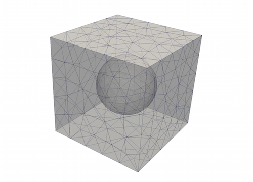
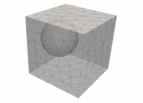
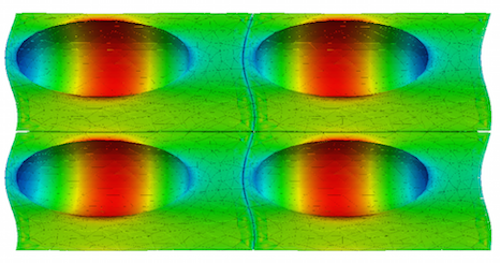
We consider periodic microstructure for which two unit cells are defined, with a central void (c) and with an off centre void (o). It is assumed that the material is elastic and subjected to small strains only.
The unit cell geometry and material properties are defined by the following Cubit journal file.
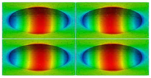
In the following figures you can see that both unit cells with void in the centre and off-centre led to the same overall material response. Once the unit cell is repeated and subjected to deformation, both solutions led to the same overall stress distribution.
The solution error is calculated from
\[ err = \frac{|\sigma_{xx}^{M,\textrm{ref}}-\sigma^M_{xx}|}{|\sigma_{xx}^{M,\textrm{ref}}|} \]
where \(\sigma^M_{xx}\) is the homogenised macroscopic stress, \(\sigma_{xx}^{M,\textrm{ref}}\) is the reference macroscopic stress. Such an error measure is equivalent to the seminorm in \(H^1(\Omega)\). The macro-stress is calculated by averaging micro-stresses as follows
\[ {\boldsymbol\sigma}^M = \frac{1}{V}\int_\Omega {\boldsymbol\sigma} \textrm{d}V = \frac{1}{V}\int_\Gamma \mathbf{x}\otimes\mathbf{t} \textrm{d}\Gamma \]
where \({\boldsymbol\sigma}\) is the micro-stress, \(\mathbf{t}\) is the traction on RVE boundary and \(\mathbf{x}\) is the spatial position on RVE surface. The reference solution has been calculated case of the unit cell with a central void, with periodic boundary conditions enforced by the Lagrange multiplier method on tetrahedral mesh with 29010 nodes and using 3rd order polynomial, this gives in total 738144 DOF. The following figure is focussed on convergence, with \(\gamma=10^{-4}\) and \(\phi=-1\).
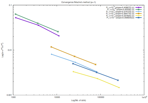
In the above figure it is shown that two types of unit cell converge to the same solution, moreover the slope of convergence for macro-stress is approximately ~0.4 for h-refined meshes. However, it is noted that mesh refinement is not-uniform and subsequent mesh refinements improve geometry approximations of the void surface. In [27] and [36] is shown that a priori error estimator has a constant which depends not only on the mesh density but also the value of the stabilisation parameter \(\gamma_0\), showing that the rate of convergence is improved for smaller values of \(\gamma_0\).
In the two following figures it is shown how convergence changes for different values of \(\gamma_0\) and \(\phi\). Two cases are considered, p- adapativity and h- non-uniform mesh refinement.
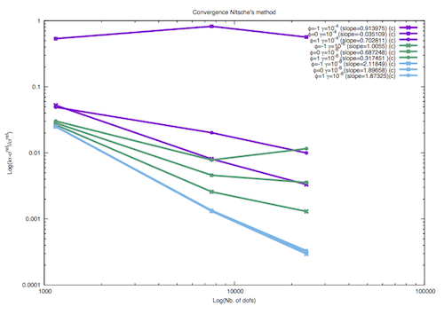
In the figure above uniform p- adaptivity is considered, three values of \(\phi = \{-1,0,1\}\) are considered and values of \(\gamma_0\) are subsequently set to 1e-4, 1e-6 and 1e-8. As shown above the convergence is unconditional for \(\phi=-1\) . Moreover convergence is lost for \(\gamma_0=10^{-4}\) and \(\phi=0\), wheres deteriorated for the symmetric case \(\phi=1\). This corresponds to the theoretical results obtained previously in Well-posedness. Moreover, it can be noted that the convergence rate improves with increasing value of \(\gamma_0\), with the value of the slope ~0.9 for \(\gamma_0=10^{-4}\), up to slope ~2.1 for \(\gamma_0=10^{-8}\). This agrees with the findings in [27] and [36].
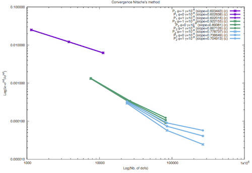
In the last figure h- adaptivity is analysed, using a constant value of \(\gamma_0=10^{-8}\) and three variants of \(\phi = \{-1,0,1\}\). It can be noted that in this case all variants showed good convergence, however for the 3rd polynomial order, convergence rate was seen to deteriorate. This is due to the large value of the stabilisation factor and the large number of DOF which reduce matrix conditioning.
The presented numerical example can be run with the script
Script needs to be run from the homogenisation build directory, i.e.
Note that the script can be easily modified, for example several values of \(\gamma_0\) can be tested.
Nitsche's method is an efficient and convenient means of enforcing multi-point constraints. The presented methodology augmented with hierarchical approximation basis and appropriate a \rm posterior error estimator gives rise to a powerful methodology. Here we limit ourself to linear constraints, however the presented approach could be easily extended to include a nonlinear constraint matrix.
The key difficulty in practical method implementation is that the Neumann terms depend on physical equations, which in general could be nonlinear. However in the implementation presented here this issue is resolved by automatic differentiation with ADOL-C, where Neumman terms are calculated for an arbitrary constitutive equation, see NitscheMethod.hpp for details.
