 |
v0.14.0 |
|
v0.14.0 |
This is an example of how to run a simultation on a cell structure, similar to what is found within wood.
Wood is a naturally occurring material, which interacts strongly with water from the air in the surrounding environment. These changes in moisture content due to the external relative humidity can cause distortions that are observable on the macro-scale. However the interactions with the water happens within the cell wall polymers, where the incoming water (solvent) is chemically bound to the polymers within through hydrogen bonding.
The transportation of this bound-water through the wood cell is a very complex process. It is not only determined by simple Fickian diffusion due to the flux of the chemical potential of the air/water in the environment, but the rate can also be controlled by the rate at which the polymer substrate deforms viscoelastically. The question of whether or not the moisture transport through these polymers is viscoelastically limited has been widely debated in the literature [74]. Using the polymeric gelmodel, in the form of a wood cell, we can determine numerically whether or not viscoelastically limited solvent uptake occurs within the amorphous polymers within wood.
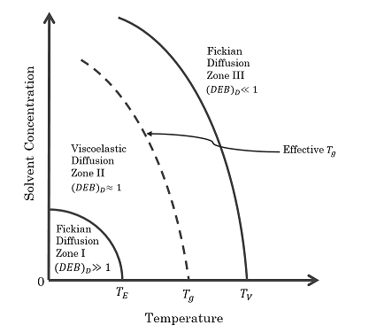
The following graph demonstrates the principles of viscoelastically limited solvent migration using the principle of the Deborah number. When the Deborah number (DEB_D) is close to 1 the diffusion and relaxation times are almost equal and it is around this region that the viscoelastic process controls the diffusion of bound-water through the sample. In this case the material temperatures are thought of as concentration dependent as we are dealing with isothermal conditions. TE is the temperature, below which the polymer acts as an elastic solid, and is characterised by a very stiff viscous damper. Tv is temperature above which the polymer acts as a viscous liquid and Tg is the glass transition temperature where the material behaviour switches from glassy to rubbery. The Deborah number is given as follows:
\[ DEB_D = \frac{T}{t} \]
where t is the time for diffusion to occur and T is the viscoelastic relaxation time, defined as follows:
\[ T = \frac{\hat{G}^\beta}{G^\beta} \]
The model used is based upon the theory of concurrent poro-elastic and viscoelastic swelling within polymeric gels by Yuhang Hu and Zhigang Suo. Viscoelasticity and poroelasticity in elastomeric gels. Acta Mechanica Solida Sinica, Vol. 25, No. 5 [32]. Further details on the mechanical model can be found in Mechanical model.
The wood cell is composed of a mixture of hemicelluloses and lignin, with the properties obtained from a paper which determines the viscoelastic properties of wood polymers using multi-scale modelling [25]. There properties are based upon a moisture content of around 10% within the wood, and as such we assign the environment to around 40% relative humidity. The shear modulus of the hemicellulose and lignin mixture is taken as 3.7 GPa, which is split evenly across the two springs, and the dashpot shear modulus is taken as 96 GPa.s. The diffusivity of bound water is taken as 1 e-05 mm2/s and the size of 1 mole of water is taken 18000 mm3. The permeability is set using the equation for diffusivity.
Above file can be found $GEL_MODULE_DIRECTORT/gel_config_cell.in
The wood cell is exposed to an environment of increased relative humidity, where the incoming water vapour is allowed to diffusive into the wood cell in the form of bound-water. The influx of bound-water comes through the lumens within the cell.
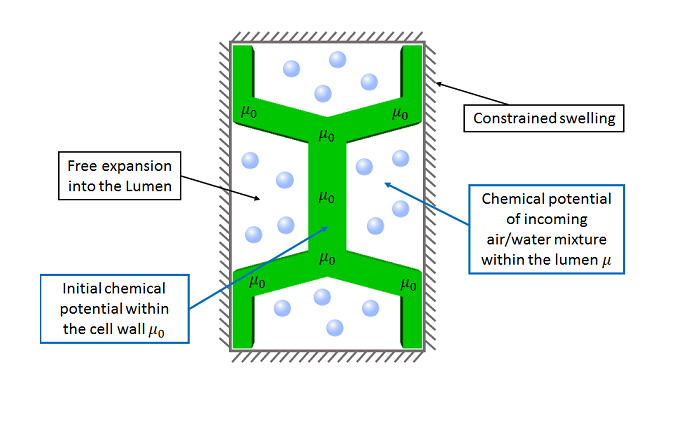

The cell is constrained in the x and y directions, with the primary mode for adsorption and desorption being expansion into, or expansion out from, the lumen within the cell. This replicated the cell being within a large network of cells tightly packed together.
The change in relative humidity is applied slowly, with a simple 1D bar problem being solved to determined the evolution of the chemical potential through a sample observable on the macro-scale, with the diffusion coefficient being set to that of water vapour through wood, 2 e-03 mm2/s.
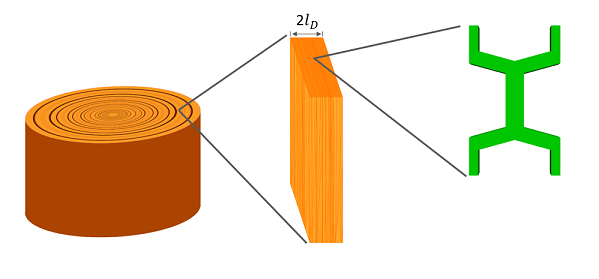
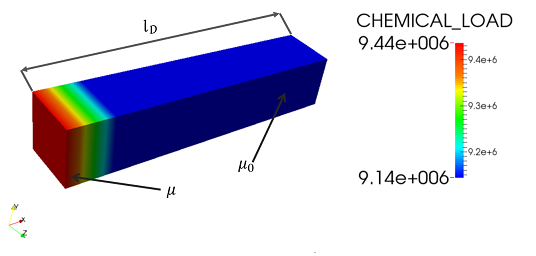
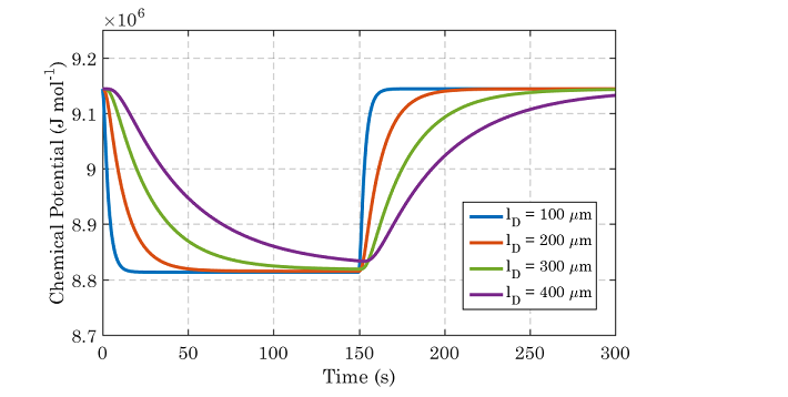
The test is carried out for several lengths of diffusion, however within this example we focus on a length of 100 micrometers. The time series for chemical potential can then be applied as a dirichlet BC within the lumens using a history file. This file can be found in $GEL_MODULE_DIRECTORT/my_chemical_history_cell.in. The history file is very long so it will not appear in this documentation, however examples an example on history files can be found in Boundary Conditions.
The chemical load history contains two columns, the left hand column is the time and the right hand column is the factor which the boundary chemical potential is multiplied by. In this case the reference boundary conditions is \mu = 3989505 J mol-1.
The boundary conditions can be calculated as shown in Dirichelt boundary condition for chemical potential
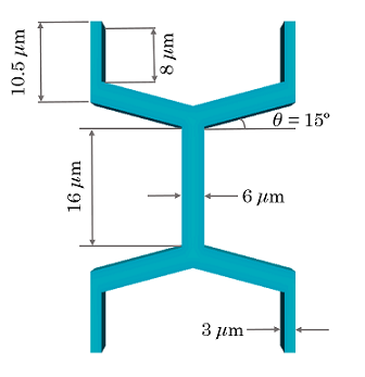
The mesh is genrated using the following script:
The mesh file used in this example is located in $MODULE_DIRECTORY/meshes/wood_cell_example.cub
The journal file used in this example is located in $MODULE_DIRECTORY/meshes/wood_cell_example.jou
Notes:
Running dynamic analysis out_values_1.h5m, out_values_2.h5m, ... are created for each time step. Post-processing mesh in output fails is stored in native MoAB data format using standard h5m.
VTK files can be generated using script located in users_modules/nonlinear_elasticity/do_vtk.sh. For example
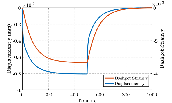
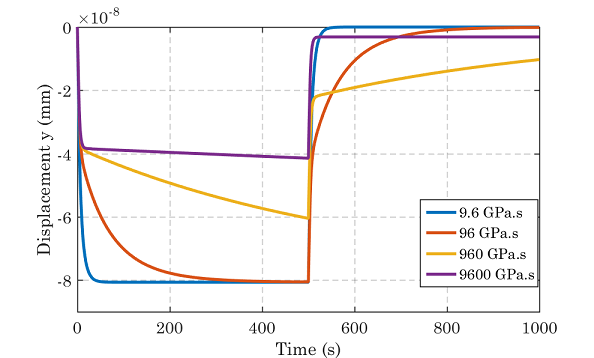
The results of the test confirm the theory of viscoelastically limited solvent migration within wood polymers. Several different values of dashpot shear modulus are used to compare the time for equilibrium. In the case where the dashpot modulus is less than the value assigned in the config file, the uptake of moisture happens much fast, behaving in a Fickian manner. The rest of the results all display different degrees of viscoelastic solvent migration. This is evidence of the models ability to capture complex phenomena within natural cell wall polymers in wood and other cellulosic materials.
It is hoped that this gel model can be applied to more complex multi-scale problems within wood and other natural ligno-cellulosic materials. It can also be applied to sorption theory, including the analysis of sorption hysteresis etc. Future documentation will be provided for this.
To download the gel model visit: https://bitbucket.org/likask/mofem_um_gels
For reference on how to apply to multi-layered materials, as is found within wood cells, see Layered Gel Problem (Response to an Environmental Change).
