 |
v0.16.0 |
Loading...
Searching...
No Matches
|
v0.16.0 |
This tutorial focuses on the theory behind the implementation of biphasic linear poroelasticity in MoFEM. The strong form and boundary conditions are defined for each phase and the weak form derived using a standard formulation for the solid phase and mixed formulation for the fluid phase. The resulting system of linearised equations are solved using the Newton-Raphson method and organised into a system of equations implemented in MoFEM.
A mixed formulation for the fluid phase is employed to mitigate instability in the pressure and fluid flux fields observed in standard formulations; often caused by a failure of the finite element method to handle instantaneous loading and abrupt material property changes. Through the introduction of an additional field for fluid flux, the formulation will improve the accuracy of flux computation. The pressure is approximated in a discontinuous space providing the capacity to compute abruptly changing pressure. Firstly, the solid phase is governed by the balance of internal and external forces. The balance of linear momentum is as follows:
\[ \begin{align} \nabla \cdot \pmb{\sigma}_A = \pmb{f} \label{eq:traction_b} \end{align} \]
where \(\pmb{\sigma}_A\) is the total (or actual) stress, \(\nabla \cdot\) is the divergence operator and \(\pmb{f}\) represents the total external force. The actual stress can be broken down into contributions from both the solid matrix, \(\pmb{\sigma}\), and pore fluid pressure, \(p\):
\[ \begin{align} \pmb{\sigma}_A = \pmb{\sigma} - \alpha p \pmb{I} \label{eq:stressbreakdown1} \end{align} \]
Here \(\alpha\) is the dimensionless Biot coefficient which measures, in a compressed medium in which water can escape, the ratio of the volume of water squeezed out to the volume change [14]. The stress within the solid matrix, \(\pmb{\sigma}\), also known as the effective stress, is defined linearly using Hooke's law:
\[ \begin{align} \pmb{\sigma} &= \mathbb{D} \epsilon \label{eq:traction_c} \\ \epsilon &= \nabla^s \pmb{u} \label{eq:traction_e} \\ \pmb{\sigma} &= \mathbb{D} \nabla^s \pmb{u} \label{eq:traction_d} \end{align} \]
where \(\mathbb{D}\) is the elasticity matrix, \(\epsilon\) is strain, and \(\nabla^s\pmb{u}\) is the symmetric gradient of displacement. The stiffness matrix follows linear elastic deformation, and is calculated using two elastic constants, Young's modulus, \(E\) and Poisson's ratio, \(\nu\) which are measures of the material properties of the solid matrix under drained conditions [70]. For an isotropic, linear elastic material, \(\mathbb{D}\) can be defined (in Voigt notation):
\[ \begin{align} \mathbb{D} = \frac{E}{(1+\nu)(1-2\nu)} \begin{bmatrix} 1-\nu & \nu & \nu & 0 & 0 & 0 \\ \nu & 1-\nu & \nu & 0 & 0 & 0 \\ \nu & \nu & 1-\nu & 0 & 0 & 0 \\ 0 & 0 & 0 & \frac{1-2\nu}{2} & 0 & 0 \\ 0 & 0 & 0 & 0 & \frac{1-2\nu}{2} & 0 \\ 0 & 0 & 0 & 0 & 0 & \frac{1-2\nu}{2} \end{bmatrix} \label{elasticitymatrix} \end{align} \]
To describe the fluid behaviour, Hooke's law will be coupled with Biot's fluid continuity equation and Darcy's law [27], the latter of which describes the fluid flow through a fully saturated, porous medium:
\[ \begin{align} \pmb{q} = -k \nabla p \label{eq:darcylaw} \end{align} \]
where \(\pmb{q}\) is the fluid flux vector, \(k\) is the isotropic permeability coefficient which has units \(m^4/Ns\), and \(p\) is the pore fluid pressure. The fluid continuity equation is as follows:
\[ \begin{align} C \dot{p} + \nabla \cdot \pmb{q} - \alpha \text{tr} \dot{\epsilon} = 0 \label{eq:fluidcontent} \end{align} \]
The storage coefficient \(C\) is measured in \(MPa^{-1}\) and is the inverse of the Biot modulus \(M\) [43], defined in Biot's Theory of Porous Media (TPM) [13]. Biot's modulus, \(M\) is a measure of, in a pressurised medium with constant volume, the amount of water which can be drawn into a soil. Therefore, the fluid continuity equation is seen as the balance of \(C\dot{p}\), the amount of fluid which can be injected into a material of fixed volume, and the amount of fluid which can escape \(\alpha \text{tr}\dot{\varepsilon}\) [70]. Detournay et al. [30] explain that Biot's two constants \(\alpha\) and \(C\) are related to the drained bulk modulus \(K\), solid bulk modulus \(K_s\), fluid bulk modulus \(K_f\) and the porosity, \(\phi\), using the following equations:
\[ \begin{align} \alpha &= 1 - \frac{K}{K_s} \\ C &= \frac{\phi}{K_f} + \frac{\alpha - \phi}{K_s} \label{eq:alphaandc} \end{align} \]
Shown by the dependency of \(\alpha\) and \(C\) on the bulk modulus, the compressibility of both the solid and fluid constituents has a direct impact on the values of the Biot coefficent and modulus. A simplification often made in poromechanical frameworks is the assumption of incompressibility of both the solid matrix and interstitial fluid. Despite this, the overall biphasic material is considered compressible: volume exchange is allowed as the material gains or loses fluid [57]. Modelling the solid and fluid constituents as incompressible leads to the respective conditions:
\[ \begin{align} K_s \rightarrow \infty \quad \Rightarrow \quad \alpha \approx 1 \\ K_f \rightarrow \infty \quad \Rightarrow \quad C \approx 0 \label{eq:compresibility1} \end{align} \]
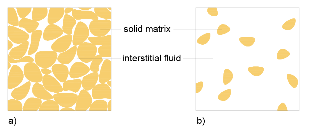
Modelling a compressible fluid, as shown in the work of [1] leads to a large reduction in the initial settlement. On the other hand, modelling the solid as compressible has the opposite effect, accelerating the consolidation process. Shown in Figure 1 is the microstructure model of a medium consisting of a solid matrix and interstitial fluid for two levels of porosity.
The form of Darcy's law varies in different applications. Darcy's law in the previous section takes the following form:
\[ \begin{align} q = -k \, \nabla p \label{eq:darcybio2} \end{align} \]
which uses the isotropic permeability coefficient, \(k\), measured in \(m^4/Ns\), a measure of the ability of a porous material to pass fluid [43]. Here, \(\nabla p\) represents the pressure gradient measured in \(N/m^3\). The following equation connects the isotropic permeability coefficient to other key fluid parameters such as intrinsic permeability and fluid density \(\rho_f\).
\[ \begin{align} k = \frac{\kappa}{\mu_f} = \frac{K_h}{\rho_{f} g} \label{eq:k12} \end{align} \]
where \(K_h\) is the hydraulic conductivity measured in \(m/s\), \(\kappa\) the intrinsic permeability measured in \(m^2\) and \(\mu_f\) the dynamic viscosity of the fluid measured in \(Ns/m^2\). On the other hand, Darcy's law incorporates the hydraulic conductivity \(K_h\) in formulations such as that by [17]. Hydraulic conductivity ( \(m/s\)) and \(\nabla h\), the dimensionless hydraulic gradient are represented as follows:
\[ \begin{align} q = -K_h \, \nabla h \label{eq:darcygeo} \end{align} \]
Implementing the hydraulic gradient into the fluid continuity equation (Equation \eqref{eq:fluidcontent}) would lead to the following re-formulation:
\[ \begin{align} C \rho_f g \dot{h} + \nabla \cdot \pmb{q} - \alpha \text{tr} \dot{\epsilon} = 0 \label{eq:fluidgeo} \end{align} \]
These two equations can be introduced into the strong form and solved in terms of hydraulic head, \(h\), which is the sum of the fluid pressure head and the head associated with elevation [40]. This form of Darcy's flow is applicable to particular geotechnical scenarios such as the seepage analysis of dams and aquifers. Here calculating the hydraulic head is essential as it is this difference in elevation of water levels which causes the flow of the fluid [38].
In this model the pressure gradient is utilised as the calculation of the pore pressure is vital for both biomedical and geotechnical applications studied. In biomechanics the variation of pressure along the intervertebral disc is crucial to understanding the distribution of stress in space and over time as well as the fracture potential of the disc. In geotechnics, fluid pressure allows for an understanding of the effective stress in soils which influences the soil behaviour under loading, helping to predict soil stability.
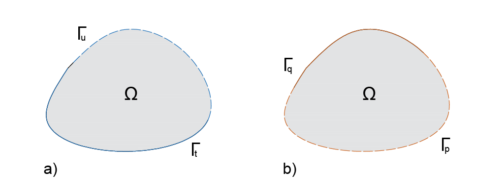
A body \(\Omega\), depicted in Figure 2, has two sets of boundary conditions — one referring to the solid matrix and the other to the pore fluid. The boundary conditions are independently defined for each subproblem. The following expressions hold for the solid boundary conditions: \(\partial \Omega = \Gamma_{u} \cup \Gamma_{t}\) and \(\Gamma_{u} \cap \Gamma_{t} = \emptyset\). The latter prohibits both Dirichlet and Neumann boundary conditions applying to a point simultaneously whilst acting over the boundary. The fluid boundary is described with \(\partial \Omega = \Gamma_{p} \cup \Gamma_{q}\), and \(\Gamma_{p} \cap \Gamma_{q} = \emptyset\). The strong form of the coupled problem is now stated, in which \(X\) represents the undeformed configuration [26].
\[ \begin{align} \notag \text{Given}\quad \quad \bar{\pmb{u}} : \Gamma_{u} \to \mathbb{R}^d, \quad \bar{\pmb{t}} : \Gamma_{t} &\to \mathbb{R}^d, \quad \bar{\pmb{q}} : \Gamma_{\bar{\pmb{q}}} \to \mathbb{R}, \quad \text{and} \quad \bar{p} : \Gamma_{\bar{p}} \to \mathbb{R}, \\ \notag \text{find} \quad \pmb{u} : \Omega \times (0,t] \to \mathbb{R}^d \quad \text{and} \quad p : \Omega \times (0,t] &\to \mathbb{R} \quad \text{such that:} \end{align} \]
\[ \begin{align} \nabla \cdot (\pmb{\sigma} - \alpha p \pmb{I}) = \pmb{0} \quad\quad\text{in}\, \Omega \label{eq:strong_a} \\ C \dot{p} + \nabla \cdot \pmb{q} - \alpha \text{tr} \dot{\epsilon} = 0 \quad\quad\text{in}\, \Omega \label{eq:strong_b} \\ \pmb{q} = -k \nabla p \quad\quad\text{in}\, \Omega \label{eq:strong_c} \\ p|_{t=0} = p_0 \quad \text{in } \Omega \label{eq:initial_condition} \end{align} \]
\[ \begin{align} \pmb{u} &= \bar{\pmb{u}} \quad \text{on } \Gamma_u \label{eq:boundary_a} \\ p &= \bar{p} \quad \text{on } \Gamma_p \label{eq:boundary_b} \\ (\pmb{\sigma} - \alpha p \pmb{I}) \pmb{n} &= \bar{\pmb{t}}\quad \text{on } \Gamma_t \label{eq:boundary_c} \\ \pmb{q} \cdot \pmb{n} &= \bar{q} \quad \text{on } \Gamma_q\label{eq:boundary_d} \end{align} \]
Equation \eqref{eq:strong_a} refers to the balance of linear momentum in the solid medium, neglecting body forces. Equation \eqref{eq:strong_b} is the mass conservation equation for the interstitial fluid (the fluid continuity equation), and Equation \eqref{eq:strong_c} is a form of Darcy’s flow relating to the movement of the fluid through the porous solid matrix. The initial pressure condition, Equation \eqref{eq:initial_condition}, is included due to the presence of the time derivative of pressure in Equation \eqref{eq:strong_b}. Equations \eqref{eq:boundary_a} and \eqref{eq:boundary_b} refer to the Dirichlet boundary conditions, and Equations \eqref{eq:boundary_c} and \eqref{eq:boundary_d} to the Neumann boundary conditions.
The governing equations are devised based on the following assumptions [14] :
To obtain the weak form of the problem using a mixed fluid phase formulation, all three governing equations in the strong form are multiplied by respective trial functions and integrated over the domain \(\Omega\). In the fluid equations, the Dirichlet boundary condition is imposed as natural on \(\Gamma_p\) (Equation \eqref{eq:boundary_b}) and the Neumann boundary condition is imposed as essential on \(\Gamma_q\) (Equation \eqref{eq:boundary_c}), which is a characteristic of mixed formulations.
The following function spaces are introduced for the primary and secondary variables \(\pmb{u}\), \(p\), and \(\pmb{q}\) [15] :
\[ Lebesgue \,\, \text{space:} \quad L^2(\Omega) = \{ u: \Omega \rightarrow \mathbb{R} \mid \int_{\Omega} |u|^2 \, d\Omega = \|u\|^2_{L^2} < +\infty \} \]
\[ Sobolev \,\, \text{space:} \quad H^1(\Omega) = \{ u \in L^2(\Omega) \mid \nabla u \in [L^2]^d(\Omega) \} \]
\[ Raviart\text{-}Thomas \,\, \text{space:} \quad H(\text{div}; \Omega) = \{ \pmb{u} \in [L^2(\Omega)]^d \mid \text{div} \, \pmb{u} \in L^2(\Omega) \} \]
\[ \text{where } x \in \Omega \subset \mathbb{R}^d, \,\, d = 2 \text{ or } 3 \]
The following tables detail the unknown fields, test functions, and their respective function spaces used in this formulation. The term \(d\) refers to the number of dimensions, allowing the vector fields \( \pmb{u}\) and \(\delta \pmb{u}\) to be defined using a scalar space \(H^1\). \(\pmb{u}\) and \(p\) are primary unknowns, and \(\pmb{q}\) a secondary unknown.
| Unknown Field | Function Space |
|---|---|
| \(\pmb{u}\) | \(\textbf{H}^1(\Omega) = \{\pmb{u} \in [H^1]^d(\Omega) \mid \pmb{u} = \bar{\pmb{u}} \text{ on } \partial \Omega_{\pmb{u}}\}\) |
| \(p\) | \(L^2(\Omega)\) |
| \(\pmb{q}\) | \(\mathcal{Q} = \{\pmb{g} \in H(\text{div};\Omega) \mid \pmb{g}\cdot\pmb{n} = \bar{q} \text{ on } \partial \Omega_{\pmb{q}}\}\) |
| Test Function | Function Space |
|---|---|
| \(\delta \pmb{u}\) | \(\textbf{H}^1_0(\Omega) = \{\delta \pmb{u} \in [H^1]^d(\Omega) \mid \delta\pmb{u} = 0 \text{ on } \partial\Omega_{\pmb{u}}\}\) |
| \(\delta p\) | \(L^2(\Omega) \) |
| \(\delta \pmb{q}\) | \(\mathcal{Q}_0 = \{\pmb{v} \in H(\text{div};\Omega) \mid \pmb{v} \cdot\pmb{n} = 0 \text{ on } \partial\Omega_{\pmb{q}}\}\) |
\[ \begin{align} \int_{\Omega} \nabla \delta \pmb{u} : (\pmb{\sigma} - \alpha p \pmb{I}) \, d\Omega - \int_{\Gamma_t} \delta \pmb{u} \cdot \bar{\pmb{t}} \, d\Gamma_t &= \pmb{0} \quad \forall \delta \pmb{u} \in H_0^1 (\Omega) \label{eq:weak_a} \\ - \int_{\Omega} \delta p \, C \dot{p} \, d\Omega - \int_{\Omega} \nabla \cdot \pmb{q} \, \delta p \, d\Omega + \int_{\Omega} \alpha \text{tr}(\dot{\epsilon}) \, \delta p \, d\Omega &= 0 \quad \forall \delta p \in L^2 (\Omega) \label{eq:weak_b} \\ \int_{\Omega} \frac{1}{k} \delta \pmb{q} \cdot \pmb{q} \, d\Omega - \int_{\Omega} (\nabla \cdot \delta \pmb{q}) \, p \, d\Omega + \int_{\Gamma_p} (\delta \pmb{q} \cdot \pmb{n}) \, \bar{p} \, d\Gamma_p &= 0 \quad \forall \delta \pmb{q} \in \mathcal{Q}_0 \label{eq:weak_c} \end{align} \]
Equation \eqref{eq:weak_b} has been multiplied by \(-1\) and Equation \eqref{eq:weak_c} divided by the permeability coefficient to ensure symmetry of the tangent matrix derived below.
Although this problem considers linear elasticity for the mechanical behaviour of the solid matrix, linearisation is still required due to the two-way coupling between the solid and fluid. The fluid induces mechanical changes, and the mechanical behaviour, in turn, influences the fluid response. Using the Newton-Raphson method, an initial estimate, \(\pmb{u}^0\), is updated so that the new estimate, \(\pmb{u}^0 + \Delta \pmb{u}\), is closer to the solution. This process repeats until the residual is satisfied within a defined tolerance [48]. The solution is approximated using the first-order Taylor series, where \(\pmb{R}(\pmb{u}^{i+1})\) is the residual at the current step:
\[ \begin{align} \pmb{R}(\pmb{u}^{i+1}) \approx \pmb{R}(\pmb{u}^{i}) + \pmb{K_T^i}(\pmb{u}^{i}) \cdot \Delta \pmb{u}^i = \pmb{0} \label{eq:taylorseries} \end{align} \]
Here, \(\pmb{K}_T^i\) is the tangent matrix at the \(i^{th}\) iteration and \(\Delta \pmb{u}^i\) is the solution increment. This first-order Taylor series can be rearranged to obtain the following linear system:
\[ \begin{align} \pmb{K}_T^i(\pmb{u}^{i}) \cdot \Delta \pmb{u}^i = - \pmb{R}(\pmb{u}^i) \label{eq:newtonraph} \end{align} \]
Here, \(\pmb{u}^i\) represents the last iteration of the displacement field. On the right-hand side is the residual of the previous iteration, the difference between the applied and internal forces [54]. The three residuals \(R_\pmb{u}(\pmb{u},p;\delta \pmb{u})\), \(R_p(\pmb{u},p,\pmb{q};\delta p)\), and \(R_\pmb{q}(p,\pmb{q};\delta \pmb{q})\) are obtained from the weak form of the solution, where each equation is set equal to zero:
\[ \begin{align} R_\pmb{u}(\pmb{u},p;\delta \pmb{u}) &= \int_{\Omega} \nabla \delta \pmb{u} : (\mathbb{D}\nabla^{s} \pmb{u} - \alpha p \pmb{I})\, d\Omega - \int_{\Gamma_t} \delta \pmb{u} \cdot \bar{\pmb{t}} \, d\Gamma_t \label{eq:residualmechanical} \\ R_p(\pmb{u},p,\pmb{q};\delta p) &= - \int_{\Omega} \delta p \, C \dot{p} \, d\Omega - \int_{\Omega} \nabla \cdot \pmb{q} \, \delta p \, d\Omega + \int_{\Omega} \alpha (\nabla^{s} \dot{\pmb{u}}):\pmb{I} \, \delta p \, d\Omega \label{eq:residualseepage1} \\ R_\pmb{q}(p,\pmb{q};\delta \pmb{q}) &= \int_{\Omega} \frac{1}{k} \delta \pmb{q} \cdot \pmb{q} \, d\Omega - \int_{\Omega} (\nabla \cdot \delta \pmb{q}) p \, d\Omega + \int_{\Gamma_p} (\delta \pmb{q} \cdot \pmb{n}) \bar{p} \, d\Gamma_p \label{eq:residualseepage2} \end{align} \]
By expanding \(R_{\pmb{u}}\) using a Taylor series, the residual can be expressed when discretised in the displacement and pressure fields. Its linearisation with respect to displacement is shown in Equation \eqref{eq:gateaux}. A similar procedure applies to the other two residuals, \(R_{p}\) and \(R_{\pmb{q}}\), with respect to pressure and flux.
\[ \begin{align} R_{\pmb{u}}(\pmb{u}_0+\Delta\pmb{u}, p_0; \delta\pmb{u}) = R_{\pmb{u}}(\pmb{u}_0,p_0;\delta\pmb{u}) + DR_{\pmb{u}}(\pmb{u}_0, p_0; \delta\pmb{u})[\Delta\pmb{u}] + O(\Delta\pmb{u}^2) \label{eq:gateaux} \end{align} \]
The higher-order term \(O(\Delta\pmb{u}^2)\) can be neglected since it approaches zero as \(\Delta\pmb{u}\) is reduced [89]. The Gâteaux derivative of the residual, \(DR(\pmb{u}_0, p_0; \delta\pmb{u})[\Delta\pmb{u}]\), is taken with respect to the change in displacement \(\Delta\pmb{u}\) at \(\pmb{u}_0\). No derivative is taken with respect to \(\nabla\pmb{u}\), as it is not an independent variable and is calculated directly using the FE framework. The Gâteaux derivatives can be approximated using Equation \eqref{eq:gateaux2} and are defined in Equations \eqref{eq:druu}–\eqref{eq:drqq}.
\[ \begin{align} DR(\pmb{u}_0, \delta \pmb{u})[\Delta \pmb{u}] = \lim_{\epsilon \to 0} \frac{R(\pmb{u}_0 + \epsilon \Delta \pmb{u}, \delta \pmb{u}) - R(\pmb{u}_0, \delta \pmb{u})}{\epsilon} \label{eq:gateaux2} \end{align} \]
\[ \begin{align} DR_{\pmb{u}}(\delta \pmb{u})[\Delta\pmb{u}] &= \int_{\Omega} \nabla \delta \pmb{u} : \mathbb{D}\nabla^{s} \Delta\pmb{u} \, d\Omega \label{eq:druu} \\ DR_{\pmb{u}}(\delta \pmb{u})[\Delta p] &= -\int_{\Omega} \nabla \delta \pmb{u} : \alpha \Delta p \pmb{I} \, d\Omega \label{eq:drup} \\ DR_{\pmb{u}}(\delta \pmb{u})[\Delta\pmb{q}] &= 0 \label{eq:druq} \\ \notag \\ DR_{p}(\delta p)[\Delta \pmb{u}] &= \int_{\Omega} \alpha (\nabla^{s} \Delta \dot{\pmb{u}}):\pmb{I} \,\delta p \, d\Omega \label{eq:drpu} \\ DR_{p}(\delta p)[\Delta p] &= - \int_{\Omega} \delta p \, C \Delta \dot{p} \, d\Omega \label{eq:drpp} \\ DR_{p}(\delta p)[\Delta\pmb{q}] &= - \int_{\Omega} \nabla \cdot \Delta \pmb{q} \, \delta p \, d\Omega \label{eq:drpq} \\ \notag \\ DR_{\pmb{q}}(\delta \pmb{q})[\Delta\pmb{u}] &= 0 \label{eq:drqu} \\ DR_{\pmb{q}}(\delta \pmb{q})[\Delta p] &= - \int_{\Omega} (\nabla \cdot \delta \pmb{q}) \, \Delta p \, d\Omega \label{eq:drqp} \\ DR_{\pmb{q}}(\delta \pmb{q})[\Delta\pmb{q}] &= \int_{\Omega} \frac{1}{k} \delta \pmb{q} \cdot \Delta \pmb{q} \, d\Omega \label{eq:drqq} \end{align} \]
The test functions and field increments are approximated using the shape functions denoted below:
| Test Function or Increment | Approximation |
|---|---|
| \(\delta \pmb{u}\) | \(\displaystyle \sum_{\beta} N_{\beta} \delta \pmb{u}_{\beta}\) |
| \(\delta p\) | \(\displaystyle \sum_{\beta} M_{\beta} \delta p_{\beta}\) |
| \(\delta \pmb{q}\) | \(\displaystyle \sum_{\beta} \pmb{Q}_{\beta} \delta q_{\beta}\) |
| \(\Delta \pmb{u}\) | \(\displaystyle \sum_{\gamma} N_{\gamma} \Delta \pmb{u}_{\gamma}\) |
| \(\Delta p\) | \(\displaystyle \sum_{\gamma} M_{\gamma} \Delta p_{\gamma}\) |
| \(\Delta \pmb{q}\) | \(\displaystyle \sum_{\gamma} \pmb{Q}_{\gamma} \Delta q_{\gamma}\) |
Substituting these into Equations \eqref{eq:druu}–\eqref{eq:drqq}, the following discretised weak form results in three residuals \(R_\pmb{u}(\pmb{u},p;\delta \pmb{u_\beta})\), \(R_p(\pmb{u},\pmb{q};\delta p_\beta)\) and \(R_\pmb{q}(p,\pmb{q};\delta \pmb{q_\beta})\):
\[ \begin{align} R_{\pmb{u}}^{\beta}(\pmb{u}, p) = \int_{\Omega} \nabla N_{\beta} : (\mathbb{D}\nabla^{s} \pmb{u} - \alpha p \pmb{I})\, d\Omega - \int_{\Gamma_t} N_{\beta} \cdot \bar{\pmb{t}} \quad d\Gamma_t \label{eq:linear1} \\ \notag \\ R_{p}^{\beta}(\pmb{u}, p, \pmb{q}) = - \int_{\Omega} M_{\beta} \, C \dot{p} \, d\Omega - \int_{\Omega} \nabla \cdot \pmb{q} M_{\beta} \, d\Omega + \int_{\Omega} \alpha (\nabla^{s} \dot{\pmb{u}}):\pmb{I} M_{\beta} \quad d\Omega \label{eq:linear2} \\ \notag \\ R_{\pmb{q}}^{\beta}(p, \pmb{q}) = \int_{\Omega} \frac{1}{k} \pmb{Q_{\beta}} \cdot \pmb{q} \, d\Omega - \int_{\Omega} (\nabla \cdot \pmb{Q_{\beta}}) p \, d\Omega + \int_{\Gamma_p} (\pmb{Q_{\beta}} \cdot \pmb{n}) \bar{p} \quad d\Gamma_p \label{eq:linear3} \end{align} \]
The respective test functions apply for all \(\delta \pmb{u_\beta}\), \(\delta p_\beta\), and \(\delta q_\beta\). These can be reduced to a saddle-point problem and expressed in matrix form.
The tangent matrix and residual vectors are defined in Equations \eqref{eq:kuu}–\eqref{eq:kqq}. Note that \(K_{\pmb{q}p}^{\beta\gamma} = [K_{p\pmb{q}}^{\beta\gamma}]^T\), which results from multiplying the weak form of the fluid equation by \(-1\) and dividing the continuity equation by \(k\).
\[ \begin{align} \begin{bmatrix} K_{\pmb{uu}}^{\beta\gamma} & K_{\pmb{u}p}^{\beta\gamma} & 0 \\ K_{p\pmb{u}}^{\beta\gamma} & K_{pp}^{\beta\gamma} & K_{p\pmb{q}}^{\beta\gamma} \\ 0 & K_{\pmb{q}p}^{\beta\gamma} & K_{\pmb{qq}}^{\beta\gamma} \end{bmatrix} \begin{bmatrix} \Delta \pmb{u^{\gamma}} \\ \Delta p^{\gamma} \\ \Delta \pmb{q^{\gamma}} \end{bmatrix} = - \begin{bmatrix} R_{\pmb{u}}^{\beta} \\ R_{p}^{\beta} \\ R_{\pmb{q}}^{\beta} \end{bmatrix} \label{mat:matrixgoverningform} \end{align} \]
\[ \begin{align} K_{\pmb{uu}}^{\beta\gamma} &= \int_{\Omega} \nabla N_{\beta} : \mathbb{D}\nabla^{s} N_{\gamma} \, d\Omega \label{eq:kuu} \\ K_{\pmb{u}p}^{\beta\gamma} &= -\int_{\Omega} \alpha \nabla N_{\beta} \cdot M_{\gamma} \pmb{I} \, d\Omega \label{eq:kup} \\ K_{p\pmb{u}}^{\beta\gamma} &= \int_{\Omega} \alpha \nabla^{s} N_{\gamma} \Delta t^{-1} : \pmb{I} M_{\beta} \, d\Omega \label{eq:kpu} \\ K_{pp}^{\beta\gamma} &= -\int_{\Omega} M_{\beta} C \Delta M_{\gamma} \Delta t^{-1} \, d\Omega \label{eq:kpp} \\ K_{p\pmb{q}}^{\beta\gamma} &= -\int_{\Omega} \nabla \cdot \pmb{Q_{\gamma}} M_{\beta} \, d\Omega \label{eq:kpq} \\ K_{\pmb{q}p}^{\beta\gamma} &= [K_{p\pmb{q}}^{\beta\gamma}]^T = -\int_{\Omega} \nabla \cdot \pmb{Q_{\beta}} M_{\gamma} \, d\Omega \label{eq:kqp} \\ K_{\pmb{qq}}^{\beta\gamma} &= \int_{\Omega} \frac{1}{k} \pmb{Q_{\beta}} \cdot \pmb{Q_{\gamma}} \, d\Omega \label{eq:kqq} \end{align} \]
Equations \eqref{eq:kpu} and \eqref{eq:kpp} contain first-order time derivatives, necessitating a time-stepping scheme. These terms originate from the Gâteaux derivatives \eqref{eq:drpu} and \eqref{eq:drpp}, which include time derivatives which are discretised in time using the PETSc TS solver, specifically the theta-method [31]. Thus the factor \(\Delta t^{-1}\) arises from this discretisation in time and represents the reciprocal of the time increment between two consecutive solution steps.
The operators used to assemble the solid matrix terms into the left-hand side matrix are:
The operators used to assemble the solid matrix terms into the right-hand side vector are:
The operators used to assemble the fluid terms into the left-hand side matrix are:
The operators used to assemble the fluid terms into the right-hand side vector are:
Finally the operators are pushed to the appropriate pipeline:
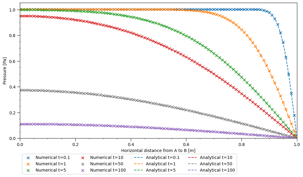
Mandel's two-dimensional soil consolidation problem is introduced in which a slab of soil is vertically compressed whilst pressure boundary conditions govern horizontal fluid flow. The known analytical solutions are used to validate the pressure solution. Thereafter an investigation is made into the dependency of the pressure solution on Biot's two fluid coefficients.
The analytical pressure solution established by [66] solves the problem of a poroelastic slab sandwiched between two rigid plates, each exerting an equal and opposite force on the slab. The lateral sides are free from normal and shear stresses and pore pressure.
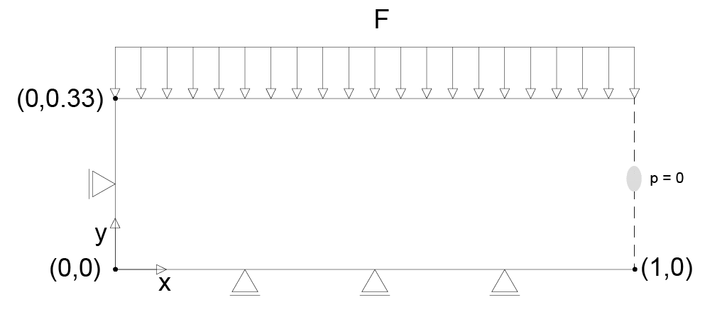
To apply a uniform displacement and force on the slab, a vertical displacement of 0.08 \(m\) is applied in the y-direction. The corresponding force, calculated from MoFEM's solution as \(1263N\), serves as the input \(F\) in the analytical solution. This successfully evades the requirement for Lagrange multipliers to enforce uniform displacement. On each side of the domain a null pressure is applied, allowing for fluid to flow out of the domain. The problem can be simplified due to \(x\) and \(y\)-symmetry to look only at the upper right quadrant, as depicted below in Figure 3. The domain consists of a \(0.33 \,\,\text{x}\,\, 1\,\,m\) rectangle with a triangular mesh. The material parameters in Table 4 match those used by Phillips [70].
| \(E\) | \(\nu\) | \(k\) | \(\alpha\) | \(C\) |
|---|---|---|---|---|
| \([Pa]\) | \([\,\,]\) | \(m^4/Ns\) | \([\,\,]\) | \(Pa^{-1}\) |
| \(1 \times 10^{4}\) | 0.2 | \(1 \times 10^{-3}\) | 1.0 | \(1 \times 10^{-1}\) |
The analytical solutions for the pressure, x and y- displacements and effective vertical stresses are as defined by Phillips [70], where \(0<n<\infty\). For comparison with MoFEM's results, the maximum value of n used is 1000.
\[ \begin{align} p &= \frac{2FB(1 + \nu_u)}{3a} \sum_{n=1}^\infty \frac{\sin \alpha_n}{\alpha_n - \sin \alpha_n \cos \alpha_n} \left( \cos \frac{\alpha_n x}{a} - \cos \alpha_n \right) \nonumber \\ &\hspace{3cm} \times \exp \left( -\frac{\alpha_n^2 c_f t}{a^2} \right) \label{eq:mandelpressuresol} \end{align} \]
Here \(\alpha_n\) represents the positive solutions to the equation:
\[ \begin{align} \tan \alpha_n = \frac{1 - \nu}{\nu_u - \nu} \alpha_n \label{eq:mandalaalphanalytical} \end{align} \]
These solutions use the additional parameters \(a\), the width of the slab, \(\mu\) shear modulus, and the fluid diffusivity \(c_f\), \(1\times10^{-3}\,N\,s/m^{2}\). The additional parameters \(B\), the dimensionless Skempton's coefficent and \(\nu_u\), undrained Poisson's ratio are as presented in [70] :
\[ \begin{align} B &= \frac{\alpha}{KC+\alpha^2} \label{eq:skempton}\\ \nu_u &= \frac{\alpha B+\nu(3-2\alpha)}{3+2\alpha B(2\nu-1)} \label{eq:undrainedmu} \end{align} \]
The effective vertical stress, which refers to the fraction of the total stress sustained by the solid skeleton, is influenced by the external stress ( \(\sigma_A\)) and interstitial pore pressure. It is calculated from the numerical results by adding the vertical (‘YY’) component of the total stress tensor to the pore pressure:
\[ \begin{align} \sigma_{YY} = \sigma_{A_{YY}} + \alpha p \label{eq:effective stress} \end{align} \]
The mesh can be created through the following Cubit journal file (mandel.jou):
After partitioning the mesh and converting to .h5m format, the following command run in the build directory will execute the poroelastic analysis in 2D.
Results:
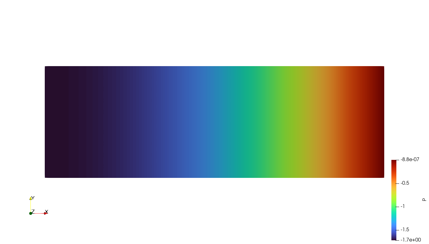
The following two figures illustrate the impact of varying the Biot modulus and storage coefficient on the pressure distribution. The Biot modulus and storage coefficient also play a significant role in the nature of poroelastic fluid flow. When considering rock types, the Biot coefficients for sandstones which typically have larger porosities range from 0.6 to 0.9 whereas for marble and granite which are less porous, the Biot coefficient is lower than 0.5 [79].
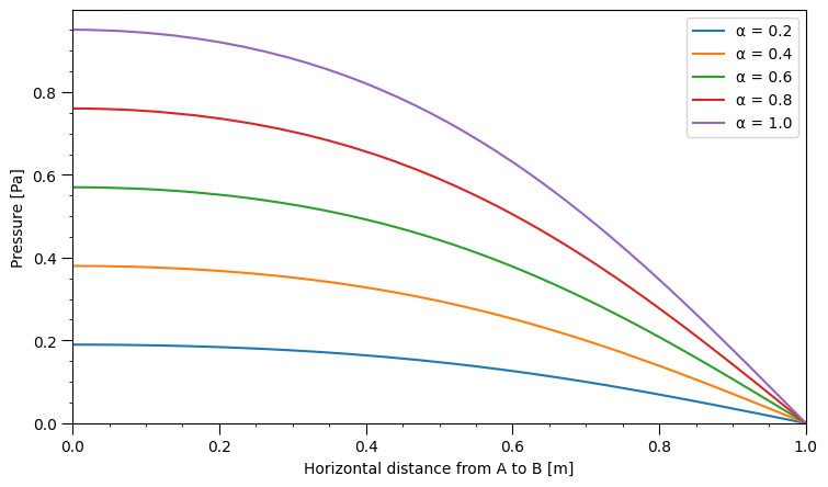
Increasing \(\alpha\) decreases consolidation, increasing the final pressure observed over the length of the domain. As \(\alpha\) is implemented in both the mechanical and seepage parts of the FE-framework, it is crucial in coordinating the two-way coupling of the porous medium.
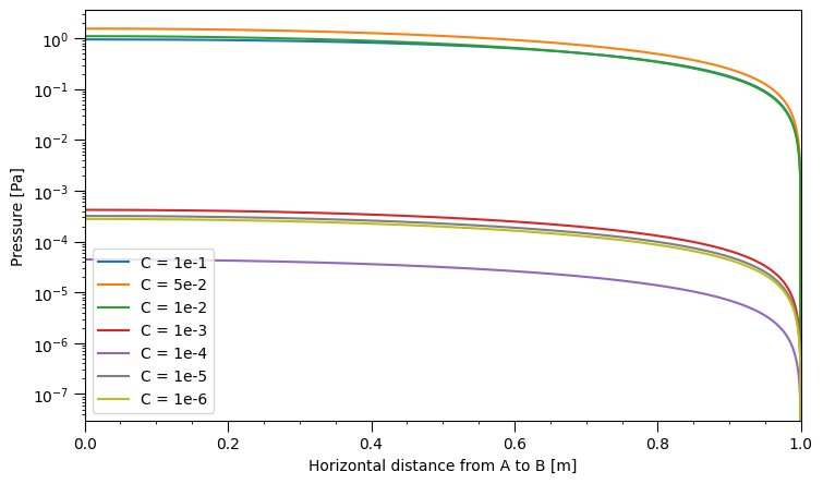
As shown in Figure 7, decreasing \(C\) by factors of 10 does not appear to have an effect on the pressure gradient at B and instead reduces the overall pore pressure, showing that the speed of fluid flow over the domain is unaffected. Decreasing \(C\) instead decreases the pressure withstood by the fluid. Reducing \(C\) does not produce a monotonic change in the pressure profile: the storage values \(1\times10^{-5}\,Pa^{-1}\) and \(1\times10^{-5}\,Pa^{-1}\) do not follow a unidirectional trend. As \(C\) approaches zero, the fluid approaches a state of incompressibility, so a possible explanation for this non-monotonic behaviour is that the solution is naturally approaching the pressure profile of an incompressible fluid as the numbers reduce in significance.
