SCL-0: Least square approximation

Table of Contents

• Introduction
• Simple Interface
• Discretisation and Operators
• Solving the problem
• Checking the results
• Visualising the results
• Plain Code

Note

Prerequisites of this tutorial include MSH-1: Create a 2D mesh from Gmsh

Note

Intended learning outcome:

• general structure of a program developed using MoFEM
• idea of Simple Interface in MoFEM and how to use it
• idea of Domain element in MoFEM and how to use it
• Use default Forms Integrators
• how to push the developed UDOs to the Pipeline
• utilisation of tools to convert outputs and visualise them in Paraview

Introduction

The aim of this tutorial is to demonstrate how MoFEM solves a simple least squares problem using a PETSc Krylov Subspace Solver (KSP). In this case, we approximate a simple analytical sinusoidal function, Eq. \eqref{eq:problemstatement}, and calculate the \(L^2\)-norm of the difference between the MoFEM approximation, \(u\), and the analytical function over a 2D domain \(\Omega\).

\[ \begin{equation} \label{eq:problemstatement} f(x,y) = \sin (10x) * \cos (10y) \end{equation} \]

The numerical approximation of the function, \(u\), is computed via the following weak form:

\[ \begin{equation} \label{eq:least_squares} \int_\Omega \delta u \, u \, \textrm{d} \Omega = \int_\Omega \delta u \, f \, \textrm{d} \Omega \quad \forall \, \delta u \in H^1(\Omega), \end{equation} \]

where \(\delta u\) is the test function and we approximate both \(u\) and \(\delta u\) in the Sobolev space \(H^1(\Omega)\), the space of square integrable functions with square integrable derivatives. There are different ways to arrive at Eq \eqref{eq:least_squares}. For example, we can minimise the square of the \(L^2\)-norm of the difference of the analytical and approximated functions:

\[ \begin{equation} \label{eq:sqnormdiff} \frac{1}{2} ||u-f||^2_{L^2} = \int_\Omega \frac{1}{2} (u - f)^2 d\Omega \end{equation} \]

To minimise it, we take the variation of this with respect to the numerical appriximation, \(u\), and set it to \(0\). Simple manipulation then suffices to recover our weak form.

Then, we check the correctness of the solution by requiring that the \(L^2\)-norm of the difference of the analytical and approximated functions be 0:

\[ \begin{equation} \label{eq:normdiff} ||u-f||_{L^2} = \left(\int_\Omega (u - f)^2 d\Omega \right)^{1/2} = 0. \end{equation} \]

Simple Interface

When reading the mesh, we use a Simple Interface. This interface will allow us to access and manipulate the mesh. Through it, we can assemble and push the operators we require for our problem. The Simple Interface also allows for mesh manipulation, so that it is possible to refine, remove degrees of freedom, and perform other operations directly through it (this tutorial does not cover these uses). The interface is accessed as follows:

MoFEMErrorCode Example::readMesh() {
  MoFEMFunctionBegin;
 
  CHKERR mField.getInterface(simpleInterface);
  CHKERR simpleInterface->getOptions();
  CHKERR simpleInterface->loadFile();
 
  MoFEMFunctionReturn(0);
}

The Simple Interface can then be used to add the field to the mesh, set the order of the fields, and set the problem up:

MoFEMErrorCode Example::setupProblem() {
  MoFEMFunctionBegin;
  // Add field
  CHKERR simpleInterface->addDomainField(FIELD_NAME, H1,
                                         AINSWORTH_LEGENDRE_BASE, FIELD_DIM);
  constexpr int order = 4;
  CHKERR simpleInterface->setFieldOrder(FIELD_NAME, order);
  CHKERR simpleInterface->setUp();
  MoFEMFunctionReturn(0);
}

Further examples of using this interface will be seen at different points of the tutorial.

Discretisation and Operators

To solve the problem, it is necessary to discretise Eq. \eqref{eq:least_squares}. We approximate the fields as follows:

\[ \begin{align} \label{eq:fields_discret} \delta u^h = \sum_{i=0}^n \delta u_i N_i, \\ u^h = \sum_{j=0}^n u_j N_j, \end{align} \]

where the superscript \(h\) denotes the approximated function, \(n\) is the number of degres of freedom, and the \(N\)s are the Hierarchical shape functions. Now, we can re-write Eq. \eqref{eq:least_squares} as:

\[ \begin{equation} \label{eq:discr_weak} \sum_{i=0}^n \sum_{j=0}^n \delta u_i \int_\Omega N_i \, N_j \, \textrm{d} \Omega \, u_j = \sum_{i=0}^n \delta u_i \int_\Omega N_i \, f \, \textrm{d} \Omega \quad \forall \, \delta u \in H^1(\Omega). \end{equation} \]

We then recast this to matrix form:

\[ \begin{equation} \label{eq:discr_mat} \textbf{K} \textbf{u} = \textbf{b}, \end{equation} \]

where the matrix and vector elements are:

\[ \begin{align} \label{eq:mat_vec} [\textrm{K}_{ij}] = \int_\Omega N_i \, N_j \, \textrm{d} \Omega, \\ [\textrm{b}_i] = \int_\Omega N_i \, f \, \textrm{d} \Omega. \end{align} \]

Now that we have our LHS and RHS, we can turn to how they are pushed to the pipeline:

MoFEMErrorCode Example::assembleSystem() {
  MoFEMFunctionBegin;
  PipelineManager *pipeline_mng = mField.getInterface<PipelineManager>();
  auto beta = [](const double, const double, const double) { return 1; };
  pipeline_mng->getOpDomainLhsPipeline().push_back(
      new OpDomainMass(FIELD_NAME, FIELD_NAME, beta));
  pipeline_mng->getOpDomainRhsPipeline().push_back(
      new OpDomainSource(FIELD_NAME, approxFunction));
  MoFEMFunctionReturn(0);
}

In this case, we are simply pushing the OpDomainMass bilinear operator to the LHS domain pipeline and the OpDomainSource linear operator to the RHS domain pipeline. We use the beta lambda function to specify constant coefficients on the Mass term in the matrix. In this case, there is no coefficient that needs to be taken into account, so we just set beta to return 1. For the RHS, approxfunction stands for the analytical function.

Solving the problem

We are now ready to solve the problem in Eq. \eqref{eq:discr_mat}. We use a KSP solver and store the solution in vector D. To create vector D, we first need a discrete manager, which we call dm and obtain directly from the Simple interface we created before. The discrete manager is a PETSc object that manages communication between the algebraic structures and the data in the mesh. In this way, we ensure that D has the correct size for our problem without actually having to specify any of its parameters ourselves. This is implemented by:

MoFEMErrorCode Example::solveSystem() {
  MoFEMFunctionBegin;
  PipelineManager *pipeline_mng = mField.getInterface<PipelineManager>();
  auto solver = pipeline_mng->createKSP();
  CHKERR KSPSetFromOptions(solver);
  CHKERR KSPSetUp(solver);
 
  auto dm = simpleInterface->getDM();
  auto D = createDMVector(dm);
  auto F = vectorDuplicate(D);
 
  CHKERR KSPSolve(solver, F, D);
  CHKERR VecGhostUpdateBegin(D, INSERT_VALUES, SCATTER_FORWARD);
  CHKERR VecGhostUpdateEnd(D, INSERT_VALUES, SCATTER_FORWARD);
  CHKERR DMoFEMMeshToLocalVector(dm, D, INSERT_VALUES, SCATTER_REVERSE);
  MoFEMFunctionReturn(0);
}
 

Checking the results

Finally, to compare the approximated and the analyitcal function, we use the following code:

MoFEMErrorCode Example::checkResults() {
  MoFEMFunctionBegin;
  PipelineManager *pipeline_mng = mField.getInterface<PipelineManager>();
  pipeline_mng->getOpDomainPostProcPipeline().clear();
  pipeline_mng->getOpDomainPostProcPipeline().push_back(
      new OpCalculateScalarFieldValues(FIELD_NAME, commonDataPtr->approxVals));
  pipeline_mng->getOpDomainPostProcPipeline().push_back(
      new OpError<FIELD_DIM>(commonDataPtr));
  CHKERR pipeline_mng->loopFiniteElementsPostProc();
  CHKERR VecAssemblyBegin(commonDataPtr->L2Vec);
  CHKERR VecAssemblyEnd(commonDataPtr->L2Vec);
  CHKERR VecAssemblyBegin(commonDataPtr->resVec);
  CHKERR VecAssemblyEnd(commonDataPtr->resVec);
  double nrm2;
  CHKERR VecNorm(commonDataPtr->resVec, NORM_2, &nrm2);
  const double *array;
  CHKERR VecGetArrayRead(commonDataPtr->L2Vec, &array);
  if (mField.get_comm_rank() == 0)
    PetscPrintf(PETSC_COMM_SELF, "Error %6.4e Vec norm %6.4e\n",
                std::sqrt(array[0]), nrm2);
  CHKERR VecRestoreArrayRead(commonDataPtr->L2Vec, &array);
  constexpr double eps = 1e-8;
  if (nrm2 > eps)
    SETERRQ(PETSC_COMM_SELF, MOFEM_DATA_INCONSISTENCY,
            "Not converged solution");
  MoFEMFunctionReturn(0);
}

Here, we reset the pipeline and push two new operators to the RHS. OpCalculateScalarFieldValues stores the values of the approximated solution in the commonDataPtr. OpError is an operator that calculates the \(L^2\) error and the norm (the square root of the error) of the difference between the approximation and analytical function and stores both values in the commonDataPtr. It is defined as follows:

template <> struct Example::OpError<1> : public DomainEleOp {
  boost::shared_ptr<CommonData> commonDataPtr;
  OpError(boost::shared_ptr<CommonData> &common_data_ptr)
      : DomainEleOp(FIELD_NAME, OPROW), commonDataPtr(common_data_ptr) {}
  MoFEMErrorCode doWork(int side, EntityType type, EntData &data) {
    MoFEMFunctionBegin;
 
    if (const size_t nb_dofs = data.getIndices().size()) {
 
      const int nb_integration_pts = getGaussPts().size2();
      auto t_w = getFTensor0IntegrationWeight();
      auto t_val = getFTensor0FromVec(*(commonDataPtr->approxVals));
      auto t_coords = getFTensor1CoordsAtGaussPts();
 
      VectorDouble nf(nb_dofs, false);
      nf.clear();
 
      FTensor::Index<'i', 3> i;
      const double volume = getMeasure();
 
      auto t_row_base = data.getFTensor0N();
      double error = 0;
      for (int gg = 0; gg != nb_integration_pts; ++gg) {
 
        const double alpha = t_w * volume;
        double diff = t_val - Example::approxFunction(t_coords(0), t_coords(1),
                                                      t_coords(2));
        error += alpha * pow(diff, 2);
 
        for (size_t r = 0; r != nb_dofs; ++r) {
          nf[r] += alpha * t_row_base * diff;
          ++t_row_base;
        }
 
        ++t_w;
        ++t_val;
        ++t_coords;
      }
 
      const int index = 0;
      CHKERR VecSetValue(commonDataPtr->L2Vec, index, error, ADD_VALUES);
      CHKERR VecSetValues(commonDataPtr->resVec, data, &nf[0], ADD_VALUES);
    }
 
    MoFEMFunctionReturn(0);
  }
};

Finally, the code checks that the norm is smaller than a tolerance and throws an error otherwise.

Visualising the results

We can run the problem by running, from the build directory,:

./approximation -json_config example.json

This will run the code and produce an output mesh called out_approx.h5m. Calling convert.py on this mesh to convert it to a vtk file, we can then visualise it in paraview as below.

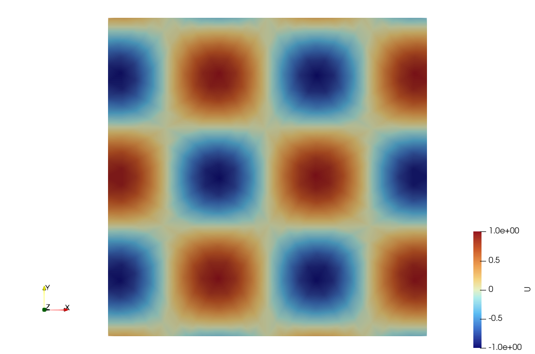
Figure 1: Output of the code.

Plain Code

/**
 * \file approximation.cpp
 * \example mofem/tutorials/scl-0_least_squares/approximation.cpp
 *
 * Using Simple interface and PipelineManager to solve least squares approximation problem.
 */
 
#include <MoFEM.hpp>
 
using namespace MoFEM;
 
static char help[] = "...\n\n";
 
#include <MoFEM.hpp>
 
constexpr char FIELD_NAME[] = "U";
constexpr int FIELD_DIM = 1;
constexpr int SPACE_DIM = 2;
 
template <int DIM> struct ElementsAndOps {};
 
template <> struct ElementsAndOps<2> {
  using DomainEle = PipelineManager::FaceEle;
};
 
template <> struct ElementsAndOps<3> {
  using DomainEle = VolumeElementForcesAndSourcesCore;
};
 
using DomainEle = ElementsAndOps<SPACE_DIM>::DomainEle;
using DomainEleOp = DomainEle::UserDataOperator;
using EntData = EntitiesFieldData::EntData;
 
using PostProcEle = PostProcBrokenMeshInMoab<DomainEle>;
 
template <int FIELD_DIM> struct ApproxFieldFunction;
 
template <> struct ApproxFieldFunction<1> {
  double operator()(const double x, const double y, const double z) {
    return sin(x * 10.) * cos(y * 10.);
  }
};
 
using OpDomainMass = FormsIntegrators<DomainEleOp>::Assembly<
    PETSC>::BiLinearForm<GAUSS>::OpMass<1, FIELD_DIM>;
using OpDomainSource = FormsIntegrators<DomainEleOp>::Assembly<
    PETSC>::LinearForm<GAUSS>::OpSource<1, FIELD_DIM>;
 
struct Example {
 
  Example(MoFEM::Interface &m_field) : mField(m_field) {}
 
  MoFEMErrorCode runProblem();
 
private:
  MoFEM::Interface &mField;
  Simple *simpleInterface;
 
  static ApproxFieldFunction<FIELD_DIM> approxFunction;
 
  MoFEMErrorCode readMesh();
  MoFEMErrorCode setupProblem();
  MoFEMErrorCode setIntegrationRules();
  MoFEMErrorCode createCommonData();
  MoFEMErrorCode boundaryCondition();
  MoFEMErrorCode assembleSystem();
  MoFEMErrorCode solveSystem();
  MoFEMErrorCode outputResults();
  MoFEMErrorCode checkResults();
 
  struct CommonData {
    boost::shared_ptr<VectorDouble> approxVals;
    SmartPetscObj<Vec> L2Vec;
    SmartPetscObj<Vec> resVec;
  };
  boost::shared_ptr<CommonData> commonDataPtr;
 
  template <int FIELD_DIM> struct OpError;
};
 
ApproxFieldFunction<FIELD_DIM> Example::approxFunction =
    ApproxFieldFunction<FIELD_DIM>();
 
//! [OpError def]
template <> struct Example::OpError<1> : public DomainEleOp {
  boost::shared_ptr<CommonData> commonDataPtr;
  OpError(boost::shared_ptr<CommonData> &common_data_ptr)
      : DomainEleOp(FIELD_NAME, OPROW), commonDataPtr(common_data_ptr) {}
  MoFEMErrorCode doWork(int side, EntityType type, EntData &data) {
    MoFEMFunctionBegin;
 
    if (const size_t nb_dofs = data.getIndices().size()) {
 
      const int nb_integration_pts = getGaussPts().size2();
      auto t_w = getFTensor0IntegrationWeight();
      auto t_val = getFTensor0FromVec(*(commonDataPtr->approxVals));
      auto t_coords = getFTensor1CoordsAtGaussPts();
 
      VectorDouble nf(nb_dofs, false);
      nf.clear();
 
      FTensor::Index<'i', 3> i;
      const double volume = getMeasure();
 
      auto t_row_base = data.getFTensor0N();
      double error = 0;
      for (int gg = 0; gg != nb_integration_pts; ++gg) {
 
        const double alpha = t_w * volume;
        double diff = t_val - Example::approxFunction(t_coords(0), t_coords(1),
                                                      t_coords(2));
        error += alpha * pow(diff, 2);
 
        for (size_t r = 0; r != nb_dofs; ++r) {
          nf[r] += alpha * t_row_base * diff;
          ++t_row_base;
        }
 
        ++t_w;
        ++t_val;
        ++t_coords;
      }
 
      const int index = 0;
      CHKERR VecSetValue(commonDataPtr->L2Vec, index, error, ADD_VALUES);
      CHKERR VecSetValues(commonDataPtr->resVec, data, &nf[0], ADD_VALUES);
    }
 
    MoFEMFunctionReturn(0);
  }
};
//! [OpError def]
 
//! [Run programme]
MoFEMErrorCode Example::runProblem() {
  MoFEMFunctionBegin;
  CHKERR readMesh();
  CHKERR setupProblem();
  CHKERR setIntegrationRules();
  CHKERR createCommonData();
  CHKERR boundaryCondition();
  CHKERR assembleSystem();
  CHKERR solveSystem();
  CHKERR outputResults();
  CHKERR checkResults();
  MoFEMFunctionReturn(0);
}
//! [Run programme]
 
//! [Read mesh]
MoFEMErrorCode Example::readMesh() {
  MoFEMFunctionBegin;
 
  CHKERR mField.getInterface(simpleInterface);
  CHKERR simpleInterface->getOptions();
  CHKERR simpleInterface->loadFile();
 
  MoFEMFunctionReturn(0);
}
//! [Read mesh]
 
//! [Set up problem]
MoFEMErrorCode Example::setupProblem() {
  MoFEMFunctionBegin;
  // Add field
  CHKERR simpleInterface->addDomainField(FIELD_NAME, H1,
                                         AINSWORTH_LEGENDRE_BASE, FIELD_DIM);
  constexpr int order = 4;
  CHKERR simpleInterface->setFieldOrder(FIELD_NAME, order);
  CHKERR simpleInterface->setUp();
  MoFEMFunctionReturn(0);
}
//! [Set up problem]
 
//! [Set integration rule]
MoFEMErrorCode Example::setIntegrationRules() {
  MoFEMFunctionBegin;
 
  auto rule = [](int, int, int p) -> int { return 2 * p; };
 
  PipelineManager *pipeline_mng = mField.getInterface<PipelineManager>();
  CHKERR pipeline_mng->setDomainLhsIntegrationRule(rule);
  CHKERR pipeline_mng->setDomainRhsIntegrationRule(rule);
 
  MoFEMFunctionReturn(0);
}
//! [Set integration rule]
 
//! [Create common data]
MoFEMErrorCode Example::createCommonData() {
  MoFEMFunctionBegin;
  commonDataPtr = boost::make_shared<CommonData>();
  commonDataPtr->resVec = createDMVector(simpleInterface->getDM());
  commonDataPtr->L2Vec =
      createVectorMPI(mField.get_comm(), (!mField.get_comm_rank()) ? 1 : 0, 1);
  commonDataPtr->approxVals = boost::make_shared<VectorDouble>();
  MoFEMFunctionReturn(0);
}
//! [Create common data]
 
//! [Boundary condition]
MoFEMErrorCode Example::boundaryCondition() { return 0; }
//! [Boundary condition]
 
//! [Push operators to pipeline]
MoFEMErrorCode Example::assembleSystem() {
  MoFEMFunctionBegin;
  PipelineManager *pipeline_mng = mField.getInterface<PipelineManager>();
  auto beta = [](const double, const double, const double) { return 1; };
  pipeline_mng->getOpDomainLhsPipeline().push_back(
      new OpDomainMass(FIELD_NAME, FIELD_NAME, beta));
  pipeline_mng->getOpDomainRhsPipeline().push_back(
      new OpDomainSource(FIELD_NAME, approxFunction));
  MoFEMFunctionReturn(0);
}
//! [Push operators to pipeline]
 
//! [Solve]
MoFEMErrorCode Example::solveSystem() {
  MoFEMFunctionBegin;
  PipelineManager *pipeline_mng = mField.getInterface<PipelineManager>();
  auto solver = pipeline_mng->createKSP();
  CHKERR KSPSetFromOptions(solver);
  CHKERR KSPSetUp(solver);
 
  auto dm = simpleInterface->getDM();
  auto D = createDMVector(dm);
  auto F = vectorDuplicate(D);
 
  CHKERR KSPSolve(solver, F, D);
  CHKERR VecGhostUpdateBegin(D, INSERT_VALUES, SCATTER_FORWARD);
  CHKERR VecGhostUpdateEnd(D, INSERT_VALUES, SCATTER_FORWARD);
  CHKERR DMoFEMMeshToLocalVector(dm, D, INSERT_VALUES, SCATTER_REVERSE);
  MoFEMFunctionReturn(0);
}
 
//! [Solve]
MoFEMErrorCode Example::outputResults() {
  MoFEMFunctionBegin;
  PipelineManager *pipeline_mng = mField.getInterface<PipelineManager>();
  auto post_proc_fe = boost::make_shared<PostProcEle>(mField);
 
  auto u_ptr = boost::make_shared<VectorDouble>();
  post_proc_fe->getOpPtrVector().push_back(
      new OpCalculateScalarFieldValues(FIELD_NAME, u_ptr));
 
  using OpPPMap = OpPostProcMapInMoab<3, 3>;
 
  post_proc_fe->getOpPtrVector().push_back(
 
      new OpPPMap(
 
          post_proc_fe->getPostProcMesh(), post_proc_fe->getMapGaussPts(),
 
          {{FIELD_NAME, u_ptr}},
 
          {},
 
          {},
 
          {})
 
  );
 
  pipeline_mng->getDomainPostProcFE() = post_proc_fe;
  CHKERR pipeline_mng->loopFiniteElementsPostProc();
  CHKERR post_proc_fe->writeFile("out_approx.h5m");
  MoFEMFunctionReturn(0);
}
//! [Postprocess results]
 
//! [Check results]
MoFEMErrorCode Example::checkResults() {
  MoFEMFunctionBegin;
  PipelineManager *pipeline_mng = mField.getInterface<PipelineManager>();
  pipeline_mng->getOpDomainPostProcPipeline().clear();
  pipeline_mng->getOpDomainPostProcPipeline().push_back(
      new OpCalculateScalarFieldValues(FIELD_NAME, commonDataPtr->approxVals));
  pipeline_mng->getOpDomainPostProcPipeline().push_back(
      new OpError<FIELD_DIM>(commonDataPtr));
  CHKERR pipeline_mng->loopFiniteElementsPostProc();
  CHKERR VecAssemblyBegin(commonDataPtr->L2Vec);
  CHKERR VecAssemblyEnd(commonDataPtr->L2Vec);
  CHKERR VecAssemblyBegin(commonDataPtr->resVec);
  CHKERR VecAssemblyEnd(commonDataPtr->resVec);
  double nrm2;
  CHKERR VecNorm(commonDataPtr->resVec, NORM_2, &nrm2);
  const double *array;
  CHKERR VecGetArrayRead(commonDataPtr->L2Vec, &array);
  if (mField.get_comm_rank() == 0)
    PetscPrintf(PETSC_COMM_SELF, "Error %6.4e Vec norm %6.4e\n",
                std::sqrt(array[0]), nrm2);
  CHKERR VecRestoreArrayRead(commonDataPtr->L2Vec, &array);
  constexpr double eps = 1e-8;
  if (nrm2 > eps)
    SETERRQ(PETSC_COMM_SELF, MOFEM_DATA_INCONSISTENCY,
            "Not converged solution");
  MoFEMFunctionReturn(0);
}
//! [Check results]
 
int main(int argc, char *argv[]) {
 
  // Initialisation of MoFEM/PETSc and MOAB data structures
  const char param_file[] = "param_file.petsc";
  MoFEM::Core::Initialize(&argc, &argv, param_file, help);
 
  try {
 
    //! [Register MoFEM discrete manager in PETSc]
    DMType dm_name = "DMMOFEM";
    CHKERR DMRegister_MoFEM(dm_name);
    //! [Register MoFEM discrete manager in PETSc
 
    //! [Create MoAB]
    moab::Core mb_instance;              ///< mesh database
    moab::Interface &moab = mb_instance; ///< mesh database interface
    //! [Create MoAB]
 
    //! [Create MoFEM]
    MoFEM::Core core(moab);           ///< finite element database
    MoFEM::Interface &m_field = core; ///< finite element database insterface
    //! [Create MoFEM]
 
    //! [Example]
    Example ex(m_field);
    CHKERR ex.runProblem();
    //! [Example]
  }
  CATCH_ERRORS;
 
  CHKERR MoFEM::Core::Finalize();
}