In this tutorial, we show how to solve nonlinear Poisson equation. Note that structure of the main program remains almost unchanged compared to linear analysis as shown in the first Poisson tutorial, i.e. COR-2: Solving the Poisson equation.
PDE problem
As a model problem for the solution of nonlinear PDEs, we take the following nonlinear Poisson equation:
\[
-\nabla \cdot (A(u)\nabla u) = f
\]
in domain \(\Omega\) with \(u=\overline{u}\) on boundary \(\partial\Omega\). The source of nonlinearity is the coefficient \(A(u)\) which is dependent on the solution \(u\), here we restrict ourself to the case
\[
A(u) = 1+u^2
\]
Note, code implementation is general, and you can look at the alternative cases, at the beginning of analytical_nonlinear_poisson.cpp example you can find two classes. Those functions can be modified to investigate alternative solutions
double operator()(
const double u) {
return 1+u*u; }
};
};
double operator()(const double u)
Note that second class has to be the exact derivative of \(A(u)\).
Linearization
With that at hand we can express equation in the weak form, where residuals are
\[
\mathbf{r}=
\left[
\begin{array}{c}
r_F\\
r_g
\end{array}
\right]=
\left\{
\begin{array}{l}
(\nabla v,(1+u^2)\nabla u)_\Omega-(v,f)_\Omega+(v,\lambda)_{\partial\Omega} = 0\\
(\tau,u-\overline{u})_{\partial\Omega} = 0
\end{array}
\right.,\quad \forall v,\tau,\; u,v \in H^1(\Omega),\;\tau,\lambda \in H^1(\partial\Omega).
\]
where \(\overline{u}\) is given function on boundary, \(f\) is a source term, \(u,\lambda\) are unknown functions and \(v,\tau\) are test functions. This notation, suitable for problems with many terms in the variational formulations, requires some explanation. First, we use the shorthand notation
\[
(v,u)_\Omega = \int_\Omega vu \textrm{d}\Omega,\quad (\lambda,u)_{\partial\Omega} = \int_{\partial \Omega} \lambda u \textrm{d}\partial\Omega
\]
With that at hand, we expand residuals in Taylor series and truncate after first order term, as a result we have
\[
\mathbf{r}^i +
\frac{\partial \mathbf{r}^i}{\partial \{ u, \lambda \}}
\left\{
\begin{array}{c}
\delta u^{i+1}\\
\delta \lambda^{i+1}
\end{array}
\right\} =
\mathbf{0}
\]
where \((\cdot)^i\) is quantity at Newton iteration \(i\), \(u^{i+1} = u^i + \delta u^{i+1}\) and \(\lambda^{i+1} = \lambda^i + \delta \lambda^{i+1}\). The linearized system of equations takes form
\[
\left\{
\begin{array}{l}
r^i_F
+
(\nabla v,(1+(u^i)^2)\nabla \delta u)_\Omega+(\nabla v,(2u^i) \nabla u^i \delta u^{i+1})_\Omega+(v,\delta\lambda^{i+1})
= 0
\\
r^i_g+
(\tau,\delta u^{i+1})_{\partial\Omega}=0
\end{array}
\right.
\]
and applying discretization
\[
u^h = \sum_i^{n_u} \phi^i(\mathbf{x}) U_i = \boldsymbol\phi\cdot\mathbf{U}
, \quad \mathbf{x} \in \Omega,\\
\lambda^h = \sum_i^{n_\lambda} \psi^i(\mathbf{x}) L_i = \boldsymbol\psi\cdot\mathbf{L}
, \quad \mathbf{x} \in \partial\Omega
\]
we get
\[
\left[
\begin{array}{c}
\mathbf{r}_F\\
\mathbf{r}_g
\end{array}
\right]+
\left[
\begin{array}{cc}
\mathbf{K}_t & \mathbf{C}^T \\
\mathbf{C} & \mathbf{0}
\end{array}
\right]
\left\{
\begin{array}{c}
\delta\mathbf{U}^{i+1}\\
\delta\mathbf{L}^{i+1}
\end{array}
\right\}
=
\left[
\begin{array}{c}
\mathbf{0}\\
\mathbf{0}
\end{array}
\right]
\]
where
\[
\mathbf{K}_t = \int_\Omega (\nabla \boldsymbol\phi)^\textrm{T} (1+(u^i)^2)\boldsymbol\phi + (\nabla \boldsymbol\phi)^\textrm{T} (2(u^i))\boldsymbol u^i \boldsymbol\phi \textrm{d}\Omega,\\
\mathbf{C} = \int_{\partial\Omega} \boldsymbol\psi^\textrm{T} \boldsymbol\phi \textrm{d}\partial\Omega,\\
\mathbf{r}_F = \mathbf{r}_{F_\Omega} + \mathbf{r}_{F_{\partial\Omega}} =
\int_\Omega (\nabla \boldsymbol\phi)^\textrm{T} (1+(u^i)^2)\boldsymbol u^i - \boldsymbol\phi^\textrm{T}f \textrm{d}\Omega+
\int_{\partial\Omega} \boldsymbol\phi^\textrm{T} \lambda^i \textrm{d}\partial\Omega\\
\mathbf{r}_g = \int_{\partial\Omega} \boldsymbol\psi^\textrm{T} (u^i-\overline{u}) \textrm{d}\partial\Omega
\]
Analytical solution
To validate correctness of implementation, we first presume exact solution to be polynomial, such that it can be precisely represented by finite element approximation base, see function
double operator()(
const double x,
const double y,
const double z)
const {
return 1+x+y+pow(z,3);
}
};
double operator()(const double x, const double y, const double t) const
where the gradient of that function is implemented here
grad(0) = 1;
grad(1) = 1;
grad(2) = 3*z*z;
return grad;
}
};
FTensor::Tensor1< double, 3 > operator()(const double x, const double y, const double t) const
and source term
double operator()(
const double x,
const double y,
const double z)
const {
return 0.4e1 + (
double) (4 * x) + (
double) (4 * y) + 0.4e1 * pow(z, 0.3e1) +
0.3e1 * (0.6e1 * z * z + 0.6e1 * (
double) x * z * z +
0.6e1 * (double) y * z * z + 0.6e1 * pow(z, 0.5e1)) * z * z +
0.6e1 * (0.2e1 + (double) (2 * x) + (double) (2 * y) +
0.2e1 * pow(z, 0.3e1) + (
double) (x * x) + (
double) (2 * x * y) +
0.2e1 * (
double) x * pow(z, 0.3e1) +
(
double) (y * y) + 0.2e1 * (
double) y * pow(z, 0.3e1) + pow(z, 0.6e1)) * z;
}
};
double operator()(const double x, const double y, const double z) const
Note that source term has a complex form and is obtained from the following formula
\[
f = \nabla \cdot \left( A(u)\nabla u \right)
\]
For 3rd polynomial order, as above, results can be obtained after tedious calculations, to avoid that you can use symbolic derivations from Mathematica, Maple, Matlab or free and open alternative Maxima.
Code dissection
Implementation of operators
All operators from this example are implemented in PoissonOperators.cpp. In particular integration is implemented in the following methods
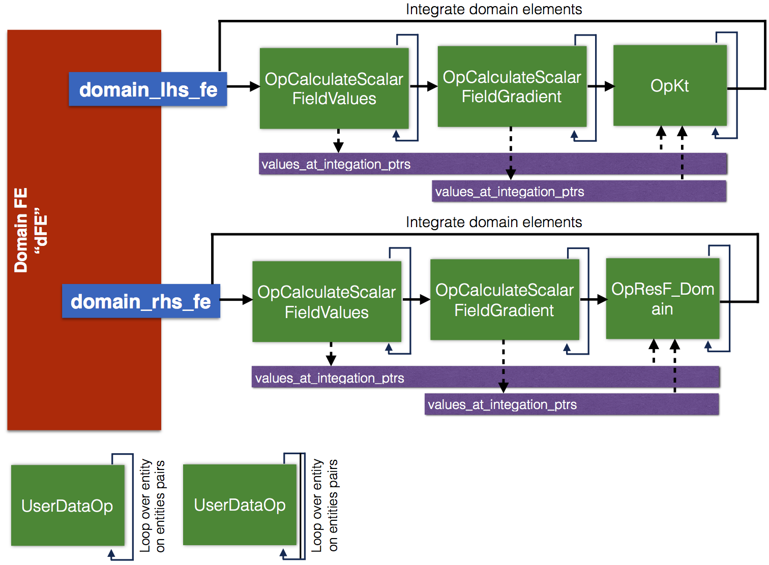
Finite element instances and setup of finite element operators, following Figure 1, is implanted in PoissonExample::CreateFiniteElements::createFEToAssembleMatrixAndVectorForNonlinearProblem, in particular we find there the following code
boost::shared_ptr<VectorDouble> values_at_integation_ptr = boost::make_shared<VectorDouble>();
boost::shared_ptr<MatrixDouble> grad_at_integation_ptr = boost::make_shared<MatrixDouble>();
domain_lhs_fe->getOpPtrVector().push_back(new OpCalculateScalarFieldValues("U",values_at_integation_ptr));
domain_lhs_fe->getOpPtrVector().push_back(new OpCalculateScalarFieldGradient<3>("U",grad_at_integation_ptr));
domain_lhs_fe->getOpPtrVector().push_back(
new OpKt(
a,diff_a,values_at_integation_ptr,grad_at_integation_ptr));
You can note that instances of vector and matrix are created to store values of function \(u^h\) and function gradients at integration points, respectively. Next operators are added to evaluate function and function gradients at integration points. Finally, operator to calculate tangent matrix is added. Operator constructor takes arguments of pointers of previously created instances of vector and matrix. The same procedure is applied to evaluate residuals by integration over domain and boundary.
Figure 1. Operators of volume finite element
Nonlinear Poisson code
#include <PoissonOperators.hpp>
static char help[] =
"...\n\n";
double operator()(
const double x,
const double y,
const double z)
const {
return 1 + x + y + pow(z, 3);
}
};
const double z) const {
grad(0) = 1;
grad(1) = 1;
grad(2) = 3 * z * z;
return grad;
}
};
double operator()(
const double x,
const double y,
const double z)
const {
return 0.4e1 + (
double)(4 * x) + (
double)(4 * y) + 0.4e1 * pow(z, 0.3e1) +
0.3e1 *
(0.6e1 * z * z + 0.6e1 * (
double)x * z * z +
0.6e1 * (double)y * z * z + 0.6e1 * pow(z, 0.5e1)) *
z * z +
0.6e1 *
(0.2e1 + (double)(2 * x) + (double)(2 * y) +
0.2e1 * pow(z, 0.3e1) + (
double)(x * x) + (
double)(2 * x * y) +
0.2e1 * (
double)y * pow(z, 0.3e1) + pow(z, 0.6e1)) *
z;
}
};
double operator()(
const double u) {
return 1 + u * u; }
};
double operator()(
const double u) {
return 2 * u; }
};
int operator()(
int,
int,
int p)
const {
return 2 * (
p + 1); }
};
int main(
int argc,
char *argv[]) {
moab::Core moab_core;
moab::Interface &moab = moab_core;
try {
PetscBool flg_test = PETSC_FALSE;
CHKERR PetscOptionsBegin(PETSC_COMM_WORLD,
"",
"Poisson's problem options",
"none");
PETSC_NULL);
CHKERR PetscOptionsBool(
"-test",
"if true is ctest",
"", flg_test,
&flg_test, PETSC_NULL);
ierr = PetscOptionsEnd();
boost::shared_ptr<ForcesAndSourcesCore>
domain_lhs_fe;
boost::shared_ptr<ForcesAndSourcesCore>
boundary_lhs_fe;
boost::shared_ptr<ForcesAndSourcesCore>
domain_rhs_fe;
boost::shared_ptr<ForcesAndSourcesCore>
boundary_rhs_fe;
boost::shared_ptr<ForcesAndSourcesCore>
domain_error;
boost::shared_ptr<PoissonExample::PostProcFE>
post_proc_volume;
boost::shared_ptr<ForcesAndSourcesCore> null;
{
domain_lhs_fe, boundary_lhs_fe, domain_rhs_fe, boundary_rhs_fe,
global_error, domain_error);
}
Simple *simple_interface;
{
CHKERR simple_interface->getOptions();
CHKERR simple_interface->loadFile();
1);
CHKERR simple_interface->addBoundaryField(
"L",
H1,
CHKERR simple_interface->addDataField(
"ERROR",
L2,
CHKERR simple_interface->setFieldOrder(
"U",
CHKERR simple_interface->setFieldOrder(
"L",
CHKERR simple_interface->setFieldOrder(
"ERROR", 0);
CHKERR simple_interface->setUp();
}
DM dm;
CHKERR simple_interface->getDM(&dm);
{
domain_lhs_fe, null, null);
boundary_lhs_fe, null, null);
domain_rhs_fe, null, null);
boundary_rhs_fe, null, null);
}
{
CHKERR DMCreateGlobalVector(dm, &F);
SNES solver;
CHKERR SNESCreate(PETSC_COMM_WORLD, &solver);
CHKERR SNESSetFromOptions(solver);
}
{
domain_error);
global_error);
if (flg_test == PETSC_TRUE) {
}
}
{
post_proc_volume);
post_proc_volume->writeFile("out_vol.h5m");
}
CHKERR VecDestroy(&global_error);
}
return 0;
}
static PetscErrorCode ierr
#define CATCH_ERRORS
Catch errors.
@ AINSWORTH_LEGENDRE_BASE
Ainsworth Cole (Legendre) approx. base .
@ L2
field with C-1 continuity
#define CHKERRG(n)
Check error code of MoFEM/MOAB/PETSc function.
#define CHKERR
Inline error check.
PetscErrorCode DMMoFEMSNESSetFunction(DM dm, const char fe_name[], MoFEM::FEMethod *method, MoFEM::BasicMethod *pre_only, MoFEM::BasicMethod *post_only)
set SNES residual evaluation function
PetscErrorCode DMMoFEMSNESSetJacobian(DM dm, const char fe_name[], MoFEM::FEMethod *method, MoFEM::BasicMethod *pre_only, MoFEM::BasicMethod *post_only)
set SNES Jacobian evaluation function
PetscErrorCode DMRegister_MoFEM(const char sname[])
Register MoFEM problem.
PetscErrorCode DMoFEMLoopFiniteElements(DM dm, const char fe_name[], MoFEM::FEMethod *method, CacheTupleWeakPtr cache_ptr=CacheTupleSharedPtr())
Executes FEMethod for finite elements in DM.
PetscErrorCode DMoFEMMeshToGlobalVector(DM dm, Vec g, InsertMode mode, ScatterMode scatter_mode)
set ghosted vector values on all existing mesh entities
const FTensor::Tensor2< T, Dim, Dim > Vec
static MoFEMErrorCode Initialize(int *argc, char ***args, const char file[], const char help[])
Initializes the MoFEM database PETSc, MOAB and MPI.
static MoFEMErrorCode Finalize()
Checks for options to be called at the conclusion of the program.
Deprecated interface functions.
MoFEMErrorCode getInterface(IFACE *&iface) const
Get interface refernce to pointer of interface.
MoFEMErrorCode createGhostVec(Vec *ghost_vec) const
MoFEMErrorCode testError(Vec ghost_vec)
Test error.
MoFEMErrorCode assembleGhostVector(Vec ghost_vec) const
Assemble error vector.
MoFEMErrorCode printError(Vec ghost_vec)
Print error.
Create finite elements instances.
MoFEMErrorCode creatFEToPostProcessResults(boost::shared_ptr< PostProcFE > &post_proc_volume) const
Create finite element to post-process results.
MoFEMErrorCode createFEToAssembleMatrixAndVectorForNonlinearProblem(boost::function< double(const double, const double, const double)> f_u, boost::function< double(const double, const double, const double)> f_source, boost::function< double(const double)> a, boost::function< double(const double)> diff_a, boost::shared_ptr< ForcesAndSourcesCore > &domain_lhs_fe, boost::shared_ptr< ForcesAndSourcesCore > &boundary_lhs_fe, boost::shared_ptr< ForcesAndSourcesCore > &domain_rhs_fe, boost::shared_ptr< ForcesAndSourcesCore > &boundary_rhs_fe, ForcesAndSourcesCore::RuleHookFun vol_rule, ForcesAndSourcesCore::RuleHookFun face_rule=FaceRule(), bool trans=true) const
Create finite element to calculate matrix and vectors.
MoFEMErrorCode createFEToEvaluateError(boost::function< double(const double, const double, const double)> f_u, boost::function< FTensor::Tensor1< double, 3 >(const double, const double, const double)> g_u, Vec global_error, boost::shared_ptr< ForcesAndSourcesCore > &domain_error) const
Create finite element to calculate error.
int operator()(int, int, int p) const
Following code is practically the same which we used to linear Poisson example. In nonlinear case, instead of KSP solver, we set-up SNES solver, first by adding finite elements instances to MoFEM SNES solver context
CHKERR DMMoFEMSNESSetJacobian(dm,simple_interface->getDomainFEName(),domain_lhs_fe,null,null);
CHKERR DMMoFEMSNESSetJacobian(dm,simple_interface->getBoundaryFEName(),boundary_lhs_fe,null,null);
CHKERR DMMoFEMSNESSetFunction(dm,simple_interface->getDomainFEName(),domain_rhs_fe,null,null);
CHKERR DMMoFEMSNESSetFunction(dm,simple_interface->getBoundaryFEName(),boundary_rhs_fe,null,null);
Once we have done this, we create solver instance and kick-start calculations
SNES solver;
CHKERR SNESCreate(PETSC_COMM_WORLD,&solver);
CHKERR SNESSetFromOptions(solver);
Note that SNES solver controls DM, and implicitly query of DM to create necessary matrices and assembly of the tangent matrix and residual vectors. SNES solver can be configured from a command line, see for details.
Running code
In order to run the program, one should first go to the directory where the problem is located, compile the code and then run the executable file. Typically, this can be done as follows
cd mofem_install/um/build/basic_finite_elements/poisson
make -j2
mpirun -np 2 ./analytical_nonlinear_poisson -file_name cube_2part.h5m -
order 3 \
-snes_monitor -snes_converged_reason -snes_type newtonls \
-snes_linesearch_type cp -snes_linesearch_monitor
where SNES options are explained here.
As a result of above command, we get
0 SNES Function norm 6.585598470492e-01
0 KSP Residual norm 6.585598470492e-01
1 KSP Residual norm 5.914941314228e-15
Line search: lambdas = [1., 0.], ftys = [-3.52513, -12.2419]
Line search terminated: lambda = 0.595591, fnorms = 0.34441
1 SNES Function norm 3.444100959814e-01
0 KSP Residual norm 3.444100959814e-01
1 KSP Residual norm 4.038504742986e-15
Line search: lambdas = [1., 0.], ftys = [-0.443111, -2.89313]
Line search terminated: lambda = 0.81914, fnorms = 0.160021
2 SNES Function norm 1.600212778450e-01
0 KSP Residual norm 1.600212778450e-01
1 KSP Residual norm 1.468413895487e-15
Line search: lambdas = [1., 0.], ftys = [-0.00392301, -0.184194]
Line search terminated: lambda = 0.978238, fnorms = 0.0159661
3 SNES Function norm 1.596606319710e-02
0 KSP Residual norm 1.596606319710e-02
1 KSP Residual norm 4.135944054060e-17
Line search: lambdas = [1., 0.], ftys = [-2.21812e-07, -0.000140473]
Line search terminated: lambda = 0.998418, fnorms = 2.23868e-05
4 SNES Function norm 2.238684200528e-05
0 KSP Residual norm 2.238684200528e-05
1 KSP Residual norm 7.619868739966e-20
Line search: lambdas = [1., 0.], ftys = [-4.35284e-16, -4.97174e-10]
Line search terminated: lambda = 0.999999, fnorms = 4.34694e-11
5 SNES Function norm 4.346943842203e-11
Nonlinear solve converged due to CONVERGED_FNORM_RELATIVE iterations 5
Approximation error 4.109e-10
Note fast convergence, after first two interactions, once iterative approximation approaches the exact solution. To obtain this solution, we are using Newton method with line-searcher, in this case, we use critical point secant line search, see details Line-search method has several alternative types and can be setup independently from solver, they can be found here.