 |
v0.14.0 |
|
v0.14.0 |
This tutorial shows how to solve the Poisson equation. We introduce the basic concepts in MoFEM and exploit the MoFEM::Simple interface to set-up the problem. A procedure is applied to the Poisson problem but can easily be modified to other problems from elasticity, fluid mechanics, thermo-elasticity, electromagnetics, etc. Methodology from this tutorial can also be applied to mix-problems, discontinuous Galerkin method or coupled problems.
We introduce fundamentals of MoFEM::Interface and MoFEM::Simple interfaces and show how to link MoFEM data structures with PETSc discrete manager. We also show how to describe fields and how to loop/iterate finite elements. This example is restricted to linear problems and the body is subjected to inhomogeneous Dirichlet boundary conditions only. We do not explain how to implement finite element data operator in this tutorial; this is part of tutorial COR-3: Implementing operators for the Poisson equation.
While writing this tutorial we don't know what type of person you are. Do you like to see examples first, before seeing the big picture? Or do you prefer to see big picture first and then look for the details after? If you are second kind, its suggested you look at MoFEM Architecture first before you start with implementation. If you like to begin with examples, skip the general details and go straight to the code.
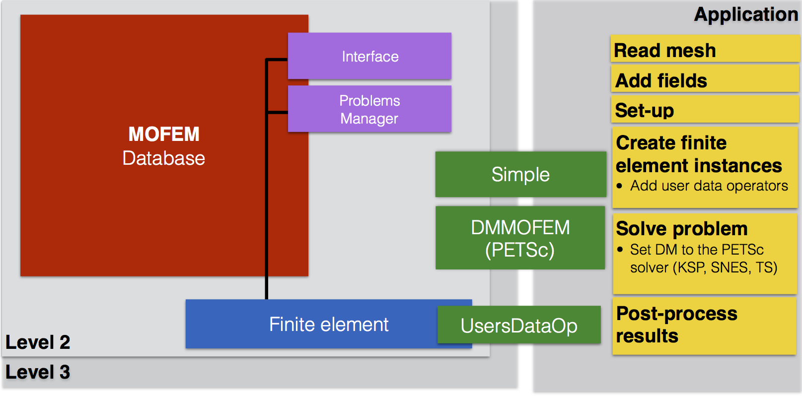
MoFEM has a bottom-up design, with several levels of abstraction, yet enables users at any level to hack levels below. This is intended to give freedom to create new methods and solve problems in new ways.
Each level up simplifies implementation, making the code shorter and easier to follow, whilst sacrificing flexibility. In this tutorial, we focus attention on functions from level 3, we are not going to describe here how the finite element is implemented, this is part of the next tutorial, COR-3: Implementing operators for the Poisson equation. In this tutorial, we focus on generic steps presented in Figure 1 below in yellow boxes.
We designed code to give you a freedom to create code which does what you want and does not force you to follow the beaten path. The implementation shown here is similar for other types of PDEs, even for nonlinear or time-dependent problems. You don't have to understand every detail of the code here, sometimes we are using advanced C++. That understanding will come later. For example, if you like to change a form of your PDE, then you need to look only how to modify differential operator to solve anisotropic the Darcy equation for flow, and that is easily done by modification of one of the operators. So, relax and look what you have below and when you are intrigued, always ask questions on our Q&A forum.
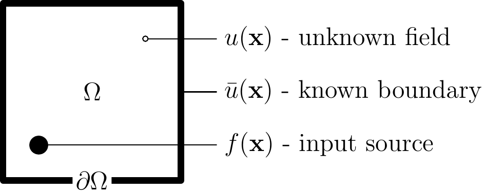
We solve the most basic of all PDEs, i.e. the Poisson equation,
\[ -\nabla^2 u(\mathbf{x}) = f(\mathbf{x}),\quad \textrm{in}\,\Omega\\ \]
where \(u=u(\mathbf{x})\) is an unknown function, \(f(\mathbf{x})\) is a given source term. The Poisson equation is in the so-called strong form, it has to be satisfied at every point of the body without boundary. To solve this PDE we need to describe the problem on the boundary, in this simple case for the purpose of the tutorial we are self-restricted to Dirichlet boundary condition where functions values are given by
\[ u(\mathbf{x})=\overline{u}(\mathbf{x}),\quad \textrm{on}\,\partial\Omega \]
where \(\overline{u}\) is prescribed function on the boundary.
The Laplacian \(\nabla^2\) in 3d space with Cartesian coordinates is
\[ \nabla^2 u(x,y,z) = \nabla \cdot \nabla u = \frac{\partial^2 u}{\partial x^2}+ \frac{\partial^2 u}{\partial y^2}+ \frac{\partial^2 u}{\partial z^2} \]
The Poisson equation arises in many physical contexts, including heat conduction, electrostatics, diffusion of substances, twisting of elastic rods, and describes many other physical problems. In general, PDE equations emerge from conservation laws, e.g. conservation of mass, electric charge or energy, i.e. one of the fundamental laws of the universe.
It is a well-established recipe how to change the equation in the form convenient for finite element calculations. The Poisson equation is multiplied by function \(u\) and integrated by parts. Without going into mathematical details, applying this procedure and enforcing constraints with Lagrange multiplier method, we get
\[ \mathcal{L}(u,\lambda) = \frac{1}{2}\int_\Omega \left( \nabla u \right)^2 \textrm{d}\Omega - \int_\Omega uf \textrm{d}\Omega + \int_{\partial\Omega} \lambda (u-\overline{u}) \textrm{d}\partial\Omega \]
where \(\lambda=\lambda(\mathbf{x})\) is Lagrange multiplier function on body boundary \(\partial\Omega\). Unknown functions can be expressed in finite dimension approximation space, as follows
\[ u^h = \sum_i^{n_u} \phi^i(\mathbf{x}) U_i = \boldsymbol\phi\cdot\mathbf{U} , \quad \mathbf{x} \in \Omega,\\ \lambda^h = \sum_i^{n_\lambda} \psi^i(\mathbf{x}) L_i = \boldsymbol\psi\cdot\mathbf{L} , \quad \mathbf{x} \in \partial\Omega \]
where \(U_i\) and \(L_i\) are unknown coefficients, called degrees of freedom. The \(\phi^i\) and \(\psi^i\) are base functions for \(u^h\) and \(\lambda^h\), respectively. The stationary point of \(\mathcal{L}(u^h,\lambda^h)\), obtained by minimalisation of Lagrangian gives Euler-Lagrange equations for discretised problem
\[ \left[ \begin{array}{cc} \mathbf{K} & \mathbf{C}^\textrm{T}\\ \mathbf{C} & \mathbf{0} \end{array} \right] \left\{ \begin{array}{c} \mathbf{U}\\ \mathbf{L} \end{array} \right\} = \left[ \begin{array}{c} \mathbf{F}\\ \mathbf{g} \end{array} \right],\\ \mathbf{K}= \int_\Omega (\nabla \boldsymbol\phi)^\textrm{T} \nabla \boldsymbol\phi \textrm{d}\Omega,\quad \mathbf{C} = \int_{\partial\Omega} \boldsymbol\psi^\textrm{T} \boldsymbol\phi \textrm{d}\partial\Omega,\\ \mathbf{F} = \int_\Omega \boldsymbol\phi^\textrm{T} f \textrm{d}\Omega,\quad \mathbf{g} = \int_{\partial\Omega} \boldsymbol\psi^\textrm{T} \overline{u} \textrm{d}\partial\Omega. \]
Applying this procedure, we transformed essential boundary conditions (in this case Dirichlet boundary conditions) into problems with only natural boundary conditions. Essential boundary conditions need to be satisfied by the approximation base. Natural conditions are satisfied while the problem is solved. Note that Lagrange multiplier has interpretation of flux here, which is in \(H^{-\frac{1}{2}}(\partial\Omega)\) space. However, in this case, the approximation of the Lagrange multiplier by a discontinuous piecewise results in a singular system of equations, since values are not bounded for natural (Neumann) boundary conditions when prescribed on all \(\partial\Omega\). For such a case, the solution is defined up to an additive constant. To remove that difficulty, we will use subspace of trace space, i.e. \(H^{-1}(\partial\Omega)\), that will generate as many constraints as many degrees of freedom for \(u^h\) on the body boundary, and thus enforce the boundary conditions exactly. For more information about spaces and deeper insight into the Poisson equation see [24], [16] and [61].
Matrices and vectors are implemented using user data operators (UDO);
We put light on the implementation of those functions in the next tutorial COR-3: Implementing operators for the Poisson equation. Here, in the following sections, we focus on the generic problem and solver setup. Complete implementation of UDO for this example is here PoissonOperators.hpp.
This example is designed to validate the basic implementation of finite element operators. In this particular case, we assume exact solution. We will focus attention on particular case for which analytical solution is given by polynomial, for example
\[ \overline{u}(\mathbf{x}) = 1+x^2+y^2+z^3 \quad \textrm{in}\Omega \]
then applying Laplacian to analytical solution we can obtain source term
\[ f(\mathbf{x}) = -4-6z. \]
If finite element approximation using 3rd order polynomials or higher, a solution of the Poisson problem is exact. In MoFEM you could easily increase the order of the polynomial, as it is shown below.
The program with comments can be accessed here analytical_poisson.cpp. In this section, we will go step-by-step through the code.
We include three header files, first with MoFEM library files and basic finite elements, second with the implementation of operators for finite elements and third with some auxiliary functions which will share tutorials about the Poisson equation.
We choose an arbitrary 3rd polynomial function, we add a function for the gradient to evaluate error on the element and a function for Laplacian to apply it as a source term in the Poisson equation.
In the following section, we initialize PETSc and construct MoAB and MoFEM databases. Starting with PETSc and MoAB
and read data from a command line argument
In this test, for simplicity, we apply approximation order uniformly. However, MoFEM in principle is designed to manage heterogeneous approximation bases.
Once we have initialized PETSc and MoAB, we create MoFEM database instance and link to it MoAB. MoFEM database is accessed by MoFEM::Interface.
Also, we need to register in PETSc implementation of MoFEM Discrete Manager.
We start with declaring smart pointers to finite element objects. A smart pointer is like a "raw" pointer, but you do not have to remember to delete allocated memory to which it points. More about shared pointers you find here, if you don't know what a pointer is, look here. You do not have to look at the details now, you can start working with code by making modifications of solutions which are already there.
Now we have to allocate memory for the finite elements and add data operators to them. We do not cover details here, this is realised by three functions, which we will use in the following tutorials
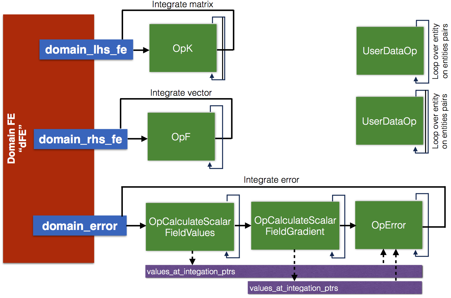
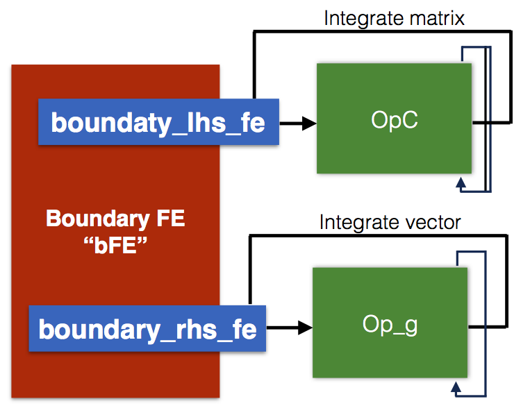
Note that those implementations are problem independent, we could use them in a different problems context. To make that more visible, we create those elements before fields and problem are defined and built. The purpose of finite elements is shown in Figure 3 and Figure 4, by users data operators added to a finite element. Finite element "domain_lhs_fe" is used to calculate the matrix by using PoissonExample::OpK, finite element "domain_rhs_fe" is used with PoissonExample::OpF. Similarly for a boundary, operators PoissonExample::OpC and PoissonExample::Op_g are used to integrate matrices and right vector for Lagrange multipliers, with finite elements "boundary_lhs_fe" and "boundary_rhs_fe", respectively. The operators MoFEM::OpCalculateScalarFieldValues, MoFEM::OpCalculateScalarFieldGradient and PoissonExample::OpError are used to integrate error in H1 norm in domain. Finite element "post_proc_volume" is used to post-process results for ParaView (or another visualization tool), it has a set of specialised operators saving results on nodes and allows to refine mesh when ho-approximation is used. The result can be stored for example on 10-node tetrahedra if needed. More details about implementation of PoissonExample::CreateFiniteElements and operators is in COR-3: Implementing operators for the Poisson equation. Basic of user data operators are explained here MoFEM Architecture.
Before we start running PETSc solver, we need to get access to DM manager, it can be simply done by
Note that user takes responsibility for deleting DM object.
Once we have DM, we add instances of previously created finite elements with their operators to DM manager, appropriately to calculate matrix and the right-hand side
At that point, we can solve the problem, applying functions exclusively from native PETSc interface
In the above code, KSP solver takes control. The KSP solver is using DM creates matrix and calls DM functions to iterate over finite elements and assembles matrix and vectors. KSP solver knows how to do it since it is using MoFEM DM which we registered at the very beginning, and get an instance of particular DM from MoFEM::Simple interface. While DM is iterating over finite elements, finite elements instance executes user data operators.
Once we have the solution, DOFs values in solution vector are scattered on the mesh
The role of MoFEM is evident here, having topology (mesh) in MoAB database, MoFEM is used to manage complexities related to problem discretization and construction of algebraic systems of equations (linear in this case). Meanwhile, PETSc manages complexities related to algebra and solution of the problem. For more details about the interaction of MoAB, MoFEM and PETSc, see MoFEM software ecosystem in MoFEM Architecture.
Finally, we can evaluate error and verify correctness of the solution
Note that function DMoFEMLoopFiniteElements takes finite element instance "domain_error" and applies it to finite element entities in the problem. For each finite element entity, finite element instance is called, and sequence of user data operators are executed on that element.
Finally, we will create a mesh for post-processing. Note that, in MoFEM, we work with spaces that not necessarily have physical DOFs at the nodes, i.e. higher order polynomials or spaces like H-div, H-curl or L2. Discontinuities on elements edges have to be shown in post-processing accurately. To resolve this issue, a set of user data operators has been created to manage those problems, see PostProcCommonOnRefMesh for details. Here, we directly run the code
In order to run the program, one should first go to the directory where the problem is located, compile the code and then run the executable file. Typically, this can be done as follows
The options are explained as follows
Initialization
MoFEM version and commit ID
MoFEM version 0.8.13 (MOAB 5.0.2 Petsc Release Version 3.9.3, Jul, 02, 2018 )
git commit id 549c206e489d605e1c9d531f5d463b99ec2adc32
Declarations
add: name U BitFieldId 1 bit number 1 space H1 approximation base AINSWORTH_LEGENDRE_BASE rank 1 meshset 12682136550675316760
add: name L BitFieldId 2 bit number 2 space H1 approximation base AINSWORTH_LEGENDRE_BASE rank 1 meshset 12682136550675316761
add: name ERROR BitFieldId 4 bit number 3 space L2 approximation base AINSWORTH_LEGENDRE_BASE rank 1 meshset 12682136550675316762
add finite element: dFE
add finite element: bFE
add problem: SimpleProblem
Set-up
Build Field U (rank 0)
nb added dofs (vertices) 180 (inactive 0)
nb added dofs (edges) 1852 (inactive 0)
nb added dofs (triangles) 1368 (inactive 0)
nb added dofs 3400 (number of inactive dofs 0)
Build Field L (rank 0)
nb added dofs (vertices) 96 (inactive 0)
nb added dofs (edges) 528 (inactive 0)
nb added dofs (triangles) 169 (inactive 0)
nb added dofs 793 (number of inactive dofs 0)
Build Field ERROR (rank 0)
nb added dofs (tets) 621 (inactive 0)
nb added dofs 621 (number of inactive dofs 0)
Nb. dofs 4814
Build Field U (rank 1)
nb added dofs (vertices) 177 (inactive 0)
nb added dofs (edges) 1814 (inactive 0)
nb added dofs (triangles) 1333 (inactive 0)
nb added dofs 3324 (number of inactive dofs 0)
Build Field L (rank 1)
nb added dofs (vertices) 99 (inactive 0)
nb added dofs (edges) 546 (inactive 0)
nb added dofs (triangles) 175 (inactive 0)
nb added dofs 820 (number of inactive dofs 0)
Build Field ERROR (rank 1)
nb added dofs (tets) 602 (inactive 0)
nb added dofs 602 (number of inactive dofs 0)
Nb. dofs 4746
Build Finite Elements dFE
id 00000000000000000000000000000001 name dFE f_id_row 00000000000000000000000000000001 f_id_col 00000000000000000000000000000001 BitFEId_data 00000000000000000000000000000101 Nb. FEs 621
id 00000000000000000000000000000001 name dFE f_id_row 00000000000000000000000000000001 f_id_col 00000000000000000000000000000001 BitFEId_data 00000000000000000000000000000101 Nb. FEs 602
Build Finite Elements bFE
id 00000000000000000000000000000010 name bFE f_id_row 00000000000000000000000000000011 f_id_col 00000000000000000000000000000011 BitFEId_data 00000000000000000000000000000011 Nb. FEs 169
id 00000000000000000000000000000010 name bFE f_id_row 00000000000000000000000000000011 f_id_col 00000000000000000000000000000011 BitFEId_data 00000000000000000000000000000011 Nb. FEs 175
Nb. entFEAdjacencies 11681
Nb. entFEAdjacencies 11480
partition_problem: rank = 0 FEs row ghost dofs problem id 00000000000000000000000000000001 FiniteElement id 00000000000000000000000000000011 name SimpleProblem Nb. local dof 4193 nb global row dofs 7868
partition_problem: rank = 0 FEs col ghost dofs problem id 00000000000000000000000000000001 FiniteElement id 00000000000000000000000000000011 name SimpleProblem Nb. local dof 4193 nb global col dofs 7868
partition_problem: rank = 1 FEs row ghost dofs problem id 00000000000000000000000000000001 FiniteElement id 00000000000000000000000000000011 name SimpleProblem Nb. local dof 3675 nb global row dofs 7868
partition_problem: rank = 1 FEs col ghost dofs problem id 00000000000000000000000000000001 FiniteElement id 00000000000000000000000000000011 name SimpleProblem Nb. local dof 3675 nb global col dofs 7868
problem id 00000000000000000000000000000001 FiniteElement id 00000000000000000000000000000011 name SimpleProblem Nb. elems 790 on proc 0
problem id 00000000000000000000000000000001 FiniteElement id 00000000000000000000000000000011 name SimpleProblem Nb. elems 777 on proc 1
partition_ghost_col_dofs: rank = 0 FEs col ghost dofs problem id 00000000000000000000000000000001 FiniteElement id 00000000000000000000000000000011 name SimpleProblem Nb. col ghost dof 0 Nb. local dof 4193
partition_ghost_row_dofs: rank = 0 FEs row ghost dofs problem id 00000000000000000000000000000001 FiniteElement id 00000000000000000000000000000011 name SimpleProblem Nb. row ghost dof 0 Nb. local dof 4193
partition_ghost_col_dofs: rank = 1 FEs col ghost dofs problem id 00000000000000000000000000000001 FiniteElement id 00000000000000000000000000000011 name SimpleProblem Nb. col ghost dof 469 Nb. local dof 3675
partition_ghost_row_dofs: rank = 1 FEs row ghost dofs problem id 00000000000000000000000000000001 FiniteElement id 00000000000000000000000000000011 name SimpleProblem Nb. row ghost dof 469 Nb. local dof 3675
Solution
0 KSP Residual norm 6.649855786390e-01
1 KSP Residual norm 6.776852388524e-14
Approximation error 2.335e-15
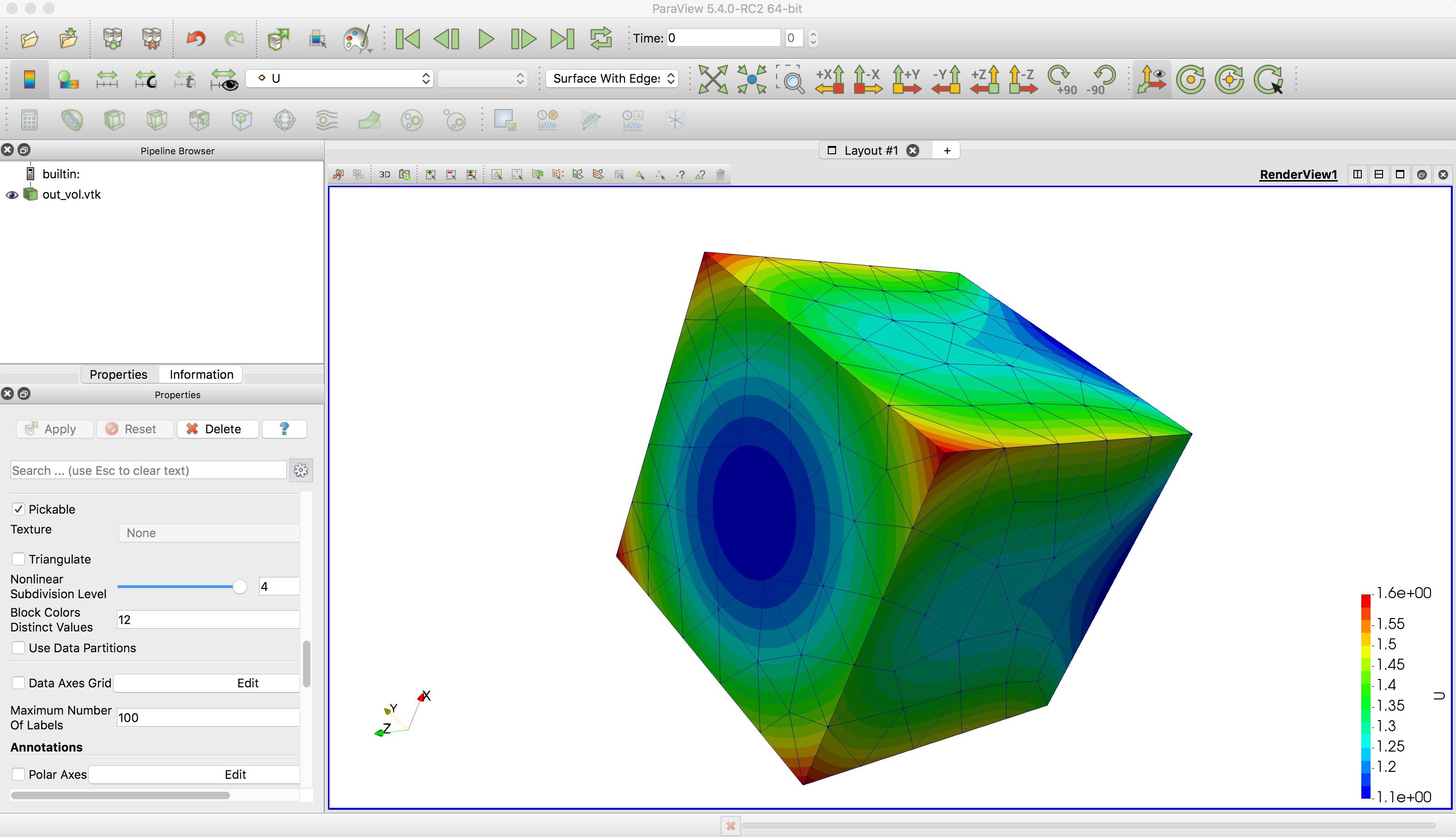
Once we have the solution, you can convert the file to VTK and open it in ParaView as shown in Figure 4
Since we are using a polynomial of 3rd order to approximate solution, results will not change if you would use coarser or finer mesh. You can generate mesh in gMesh, Salome or generate mesh in any format on the list
Format        Name                            Read    Write   File name description
-----------------------------------------------------------------------------------
MOAB          MOAB native (HDF5)              yes    yes     h5m mhdf
EXODUS        Exodus II                       yes    yes     exo exoII exo2 g gen
NC            Climate NC                      yes    yes     nc
UNV           IDEAS format                    yes     no     unv
MESHTAL       MCNP5 format                    yes     no     meshtal
NAS           NASTRAN format                  yes     no     nas bdf
Abaqus        mesh  ABAQUS INP mesh format    yes     no     abq
Atilla        RTT Mesh  RTT Mesh Format       yes     no     rtt
VTK           Kitware VTK                     yes    yes     vtk
OBJ mesh      OBJ mesh format                 yes     no     obj
SMS           RPI SMS                         yes     no     sms
CUBIT         Cubit                           yes     no     cub
SMF           QSlim format                    yes    yes     smf
SLAC          SLAC                             no    yes     slac
GMV           GMV                              no    yes     gmv
ANSYS         Ansys                            no    yes     ans
GMSH          Gmsh mesh file                  yes    yes     msh gmsh
STL           Stereo Lithography File (STL)   yes    yes     stl
TETGEN        TetGen output files             yes     no     node ele face edge
TEMPLATE      Template input files            yes    yes
You can obtain that list executing from the command line
\[ u = sin(kx) \]
where \(k\) is a small number.Please feel free to ask any questions on our Q&A forum, see link.
