v0.13.2
Loading...
Searching...
No Matches
MIX-0: Mixed formulation of Poisson equation
Note
Prerequisites of this tutorial include SCL-1: Poisson's equation (homogeneous BC) and FUN-2: Hierarchical approximation


Note
Intended learning outcome:
  • Motivation for using mixed problem formulation
  • Derivation of the mixed weak form for the Poisson equation
  • Preliminaries for function spaces L2 and H(div)
  • Implementation of the mixed weak form and error indicators
  • Convergence analysis for p-adaptive refinement

Introduction and motivation

We will start this tutorial by introducing the idea of the mixed form and its difference from the coupled problem formulation. In case of the coupled problem, we consider the interplay between two (or more) sub-problems governed by different physical equations and therefore described by two (or more) fields. Examples of coupled problems include thermoelasticity, electroelasticity, fluid-structure interaction and many others. On the contrary, mixed problem formulation is obtained upon introduction of one (or more) auxiliary variable(s) in a problem governed by one physical process. Examples of classical problems permitting (and benefiting from) such formulation are:

  • Incompressible elasticity (auxiliary variable: hydrostatic pressure)
  • Stokes/Navier-Stokes problem for viscous incompressible flow (auxiliary variable: fluid pressure)
  • Convection-Reaction-Diffusion problem (auxiliary variable: flux)
  • Mechanical contact problem (auxiliary variable: contact pressure).

There are multiple reasons for using mixed formulation, see [12] for more details:

  • Presence of constraints in a problem under study (incompressible elasticity/fluid flow, contact problem)
  • Importance of new variables appearing in the formulation (accurate computation of stresses in elastic problem and fluxes in diffusion problem)
  • Possibility to obtain weaker formulation with less requirements on the regularity of the solution
  • Embedded reliable and efficient a posteriori error estimates.

Note that in this tutorial particular attention will be given to the error estimators naturally emerging within the mixed formulation and permitting easy implementation of adaptive refinement.

Derivation of the mixed weak form for the Poisson equation

The strong form of the boundary value problem for the Poisson equation reads:

\[ \begin{align} \label{eq:poisson}-\textrm{div}\:(\nabla u) = f & \quad \textrm{in}\; \Omega \\ \label{eq:dirichlet}u = 0 & \quad \textrm{on}\; \partial\Omega, \end{align} \]

where the homogeneous Dirichlet boundary condition is imposed on the whole boundary of the domain. In order to obtain the mixed formulation, we introduce a new variable \(\mathbf{q}\) representing the flux and rewrite the statement of the problem as follows:

\[ \begin{align} \label{eq:flux}\mathbf{q} &= \nabla u & \textrm{in}\; \Omega\\ \label{eq:cont}-\textrm{div}\,\mathbf{q} &= f & \textrm{in}\; \Omega\\ \label{eq:bc}u &= 0 & \textrm{on}\; \partial\Omega. \end{align} \]

We then multiply the left and right hand sides of Eqs. \eqref{eq:flux} and \eqref{eq:cont} by test functions \(\delta\mathbf{q}\) and \(\delta u\), respectively, and integrate over the domain:

\[ \begin{align} \label{eq:flux_int}\int_{\Omega}\mathbf{q}\cdot\delta\mathbf{q}\,\textrm{d}\Omega - \int_{\Omega}\nabla u \cdot \delta\mathbf{q} \,\textrm{d}\Omega &= 0 \\ -\int_{\Omega}\textrm{div}\,\mathbf{q}\delta u \,\textrm{d}\Omega &= \int_{\Omega}f\, \delta u \,\textrm{d}\Omega \end{align} \]

We now notice that the second term in \eqref{eq:flux_int} can be integrated by parts, providing:

\[ \begin{align} \label{eq:flux_int_part}\int_{\Omega}\mathbf{q}\cdot\delta\mathbf{q}\,\textrm{d}\Omega + \int_{\Omega} u\, \textrm{div}\, \delta\mathbf{q} \,\textrm{d}\Omega -\int_{\partial\Omega} u\, \delta\mathbf{q}\cdot\mathbf{n} \,\textrm{d}\Gamma &= 0 \\ -\int_{\Omega}\textrm{div}\,\mathbf{q}\,\delta u \,\textrm{d}\Omega &= \int_{\Omega}f\, \delta u \,\textrm{d}\Omega \end{align} \]

Since \(u=0\) on \(\partial\Omega\), the boundary term in \eqref{eq:flux_int_part} vanishes. Note that in this case the Dirichlet boundary condition on the field \(u\) \eqref{eq:bc} is imposed in the sense of natural boundary condition, which is typical for mixed formulations. We arrive at the mixed weak form of the problem \eqref{eq:poisson}-\eqref{eq:dirichlet}: Find \(\mathbf{q}\in H(\textrm{div};\Omega)\) and \(u\in L^2(\Omega)\) such that

\[ \begin{align} \label{eq:weak_1}\int_{\Omega}\mathbf{q}\cdot\delta\mathbf{q}\,\textrm{d}\Omega + \int_{\Omega} u\, \textrm{div}\, \delta\mathbf{q} \,\textrm{d}\Omega &= 0 & \forall\, \delta\mathbf{q} \in H(\textrm{div};\Omega)\\ \label{eq:weak_2}\int_{\Omega}\textrm{div}\,\mathbf{q}\,\delta u \,\textrm{d}\Omega &= -\int_{\Omega}f\, \delta u \,\textrm{d}\Omega & \forall\, \delta u \in L^2(\Omega) \end{align} \]

where the following notations of function spaces were used:

\[ \begin{align} L^2(\Omega) &:= \left\{ u(\mathbf{x}) : \Omega \rightarrow R \;\left|\; \int_{\Omega}|u|^2\;\textrm{d}\Omega = ||u||^2_{\Omega} < +\infty\right.\right\} \\ H(\textrm{div};\Omega) &:= \left\{ \mathbf{q} \in [L^2(\Omega)]^2 \;\left|\; \textrm{div}\:\mathbf{u}\in L^2(\Omega)\right.\right\} \end{align} \]

As was mentioned above, one of the main benefits of the mixed formulation is associated with embedded error estimates. It is important to distinguish between error indicators which compute local measure of the error and error estimators which provide mathematically strict bounds on the global error. In this tutorial we will consider only the former, and in particular, will study a simple error indicator which represents the norm of difference between the gradient of field \(u\) and the flux \(\mathbf{q}\) computed over a finite element \(\Omega_e\), see [41] for more details:

\[ \begin{equation} \label{eq:indic}\eta_e := ||\nabla u - \mathbf{q}||_{\Omega_e}^2. \end{equation} \]

Implementation

Note that function MixedPoisson::runProblem() is shorter than in previous tutorials, e.g. SCL-1: Poisson's equation (homogeneous BC) since several functions are nested in MixedPoisson::solveRefineLoop():

MoFEMErrorCode MixedPoisson::runProblem() {
}
#define MoFEMFunctionBegin
First executable line of each MoFEM function, used for error handling. Final line of MoFEM functions ...
Definition: definitions.h:346
#define MoFEMFunctionReturn(a)
Last executable line of each PETSc function used for error handling. Replaces return()
Definition: definitions.h:416
#define CHKERR
Inline error check.
Definition: definitions.h:535
MoFEMErrorCode solveRefineLoop()
[Refine]
MoFEMErrorCode createCommonData()
[Set integration rule]
MoFEMErrorCode setIntegrationRules()
[Set up problem]
MoFEMErrorCode runProblem()
[Run programme]
MoFEMErrorCode setupProblem()
[Read mesh]
MoFEMErrorCode readMesh()
[Run programme]

Furthermore, function MixedPoisson::readMesh() is similar to the one in SCL-1: Poisson's equation (homogeneous BC) and will not be discussed here. However, the function MixedPoisson::setupProblem() has features unique to the considered problem:

MoFEMErrorCode MixedPoisson::setupProblem() {
// Note that in 2D case HDIV and HCURL spaces are isomorphic, and therefore
// only base for HCURL has been implemented in 2D. Base vectors for HDIV space
// are be obtained after rotation of HCURL base vectors by a right angle
1);
// We use AINSWORTH_LEGENDRE_BASE since DEMKOWICZ_JACOBI_BASE for triangle
// is not yet implemented for L2 space. For quads DEMKOWICZ_JACOBI_BASE and
// AINSWORTH_LEGENDRE_BASE are construcreed in the same way
CHKERR simpleInterface->addDomainField("U", L2, AINSWORTH_LEGENDRE_BASE, 1);
CHKERR PetscOptionsGetInt(PETSC_NULL, "", "-ref_iter_num", &refIterNum,
PETSC_NULL);
baseOrder = 2;
CHKERR PetscOptionsGetInt(PETSC_NULL, "", "-base_order", &baseOrder,
PETSC_NULL);
CHKERR simpleInterface->setFieldOrder("FLUX", baseOrder);
CHKERR simpleInterface->setFieldOrder("U", baseOrder - 1);
CHKERR mField.get_moab().get_entities_by_dimension(0, 2, domainEntities,
false);
Tag th_order;
CHKERR getTagHandle(mField, "ORDER", MB_TYPE_INTEGER, th_order);
for (auto ent : domainEntities) {
CHKERR mField.get_moab().tag_set_data(th_order, &ent, 1, &baseOrder);
}
}
@ AINSWORTH_LEGENDRE_BASE
Ainsworth Cole (Legendre) approx. base .
Definition: definitions.h:60
@ DEMKOWICZ_JACOBI_BASE
Definition: definitions.h:66
@ L2
field with C-1 continuity
Definition: definitions.h:88
@ HCURL
field with continuous tangents
Definition: definitions.h:86
Simple * simpleInterface
Range domainEntities
MoFEM::Interface & mField
static MoFEMErrorCode getTagHandle(MoFEM::Interface &m_field, const char *name, DataType type, Tag &tag_handle)
[Source function]
virtual moab::Interface & get_moab()=0

First, we add domain fields for the flux \(\mathbf{q}\) (choosing space HCURL) and for \(u\) (space L2). Space H(curl) in 2D is defined as:

\[ H(\textrm{curl};\Omega) := \left\{ \mathbf{q} \in [L^2(\Omega)]^2 \;\left|\; \textrm{curl}\:\mathbf{u}\in L^2(\Omega)\right.\right\} \]

It is important to note that choosing the H(curl) space for fluxes is not a mistake here. In turns out that in 2D case spaces H(div) and H(curl) are isomorphic, and therefore only base for H(curl) has been implemented in 2D. Base vectors for H(div) space can be easily obtained after rotation of H(curl) space base vectors by a right angle, see [12] for more details. Note also that bases of both H(div) and H(curl) are vectorial, and, therefore, only 1 coefficient per base function is required for vector field \(\mathbf{q}\).

Next, user-defined orders are set for the fields: if \(p\) is the order for the flux \(\mathbf{q}\in H(\textrm{div};\Omega)\), then order for the field \(u\in L^2(\Omega)\) is \((p-1)\) which is required to satisfy the inf-sup (LBB) stability conditions [12]. Finally, since in this tutorial we will discuss the implementation of adaptive p-refinement, the user-defined approximation order \(p\) is stored in the MOAB database on tags of each domain element.

Setting the integration rule in function MixedPoisson::setIntegrationRules() is similar to other tutorials:

auto rule = [](int, int, int p) -> int { return 2 * p + 1; };
PipelineManager *pipeline_mng = mField.getInterface<PipelineManager>();
CHKERR pipeline_mng->setDomainLhsIntegrationRule(rule);
CHKERR pipeline_mng->setDomainRhsIntegrationRule(rule);
}
static Index< 'p', 3 > p
MoFEMErrorCode getInterface(IFACE *&iface) const
Get interface refernce to pointer of interface.

The highest order of the integrand is found in the diagonal term in Eq. \eqref{eq:weak_1}, and therefore the rule is set to \((2 p + 1)\), where \(p\) is order of base functions for fluxes. Note that the order is increased by 1 to accommodate for the case of the higher order geometry.

As was mentioned above, functions MixedPoisson::assembleSystem(), MixedPoisson::solveSystem(), MixedPoisson::checkError() and MixedPoisson::outputResults() are nested in MixedPoisson::solveRefineLoop(). Note that first, these functions are called outside the loop:

for (int ii = 0; ii < refIterNum; ii++) {
CHKERR checkError(ii + 1);
}
}
MoFEMErrorCode assembleSystem()
[Create common data]
MoFEMErrorCode outputResults(int iter_num=0)
[Check error]
MoFEMErrorCode refineOrder()
[Solve]
MoFEMErrorCode checkError(int iter_num=0)
[Solve and refine loop]
MoFEMErrorCode solveSystem()
[Assemble system]

If user-defined number of p-refinement iterations is greater or equal to 1, then the loop starts from the refinement procedure and, subsequently, calls to MixedPoisson::assembleSystem(), MixedPoisson::solveSystem(), MixedPoisson::checkError() and MixedPoisson::outputResults() are repeated. We will now consider these functions in more detail.

Assembling the system

MoFEMErrorCode MixedPoisson::assembleSystem() {
PipelineManager *pipeline_mng = mField.getInterface<PipelineManager>();
pipeline_mng->getDomainLhsFE().reset();
pipeline_mng->getDomainRhsFE().reset();
pipeline_mng->getOpDomainRhsPipeline().clear();
pipeline_mng->getOpDomainLhsPipeline().clear();
auto det_ptr = boost::make_shared<VectorDouble>();
auto inv_jac_ptr = boost::make_shared<MatrixDouble>();
auto jac_ptr = boost::make_shared<MatrixDouble>();
pipeline_mng->getOpDomainLhsPipeline().push_back(
new OpCalculateHOJacForFace(jac_ptr));
pipeline_mng->getOpDomainLhsPipeline().push_back(
new OpInvertMatrix<2>(jac_ptr, det_ptr, inv_jac_ptr));
pipeline_mng->getOpDomainLhsPipeline().push_back(new OpMakeHdivFromHcurl());
pipeline_mng->getOpDomainLhsPipeline().push_back(
new OpSetContravariantPiolaTransformOnFace2D(jac_ptr));
pipeline_mng->getOpDomainLhsPipeline().push_back(
new OpSetInvJacHcurlFace(inv_jac_ptr));
pipeline_mng->getOpDomainLhsPipeline().push_back(new OpSetHOWeightsOnFace());
auto beta = [](const double, const double, const double) { return 1; };
pipeline_mng->getOpDomainLhsPipeline().push_back(
new OpHdivHdiv("FLUX", "FLUX", beta));
auto unity = []() { return 1; };
pipeline_mng->getOpDomainLhsPipeline().push_back(
new OpHdivU("FLUX", "U", unity, true));
auto source = [&](const double x, const double y, const double z) {
return -sourceFunction(x, y, z);
};
pipeline_mng->getOpDomainRhsPipeline().push_back(
new OpDomainSource("U", source));
}
FormsIntegrators< DomainEleOp >::Assembly< PETSC >::BiLinearForm< GAUSS >::OpMixDivTimesScalar< 2 > OpHdivU
FormsIntegrators< DomainEleOp >::Assembly< PETSC >::BiLinearForm< GAUSS >::OpMass< 3, 3 > OpHdivHdiv
FormsIntegrators< DomainEleOp >::Assembly< PETSC >::LinearForm< GAUSS >::OpSource< 1, 1 > OpDomainSource
static double sourceFunction(const double x, const double y, const double z)
[Analytical function gradient]

Assembly of the system requires first computation of the Jacobian matrix, its inverse and the determinant. Furthermore, as the H(curl) space was chosen for approximation of the flux field, the transformation of the base to H(div) space (rotation by the right angle of the base vectors) is obtained by pushing the corresponding operator. Moreover, as the base for H(div) space is vectorial, the contravariant Piola transform is required, see [12] for more details, and the associated operator is also pushed to the pipeline. Upon these preliminary steps, only three additional operators are needed to assemble the discretized version of the system \eqref{eq:weak_1}- \eqref{eq:weak_2}:

  • Operator OpHdivHdiv() is used to compute the diagonal term in \eqref{eq:weak_1};
  • Operator OpHdivU() computes off-diagonal (symmetric) terms in \eqref{eq:weak_1} and \eqref{eq:weak_2}
  • Operator OpDomainSource() assembles the source term in \eqref{eq:weak_2}.

Operators for computing error indicators

The solution of the system is implemented in MixedPoisson::solveSystem() and is similar to other tutorials. However, function MixedPoisson::checkError() deserves discussion here:

MoFEMErrorCode MixedPoisson::checkError(int iter_num) {
PipelineManager *pipeline_mng = mField.getInterface<PipelineManager>();
pipeline_mng->getDomainLhsFE().reset();
pipeline_mng->getDomainRhsFE().reset();
pipeline_mng->getOpDomainRhsPipeline().clear();
auto det_ptr = boost::make_shared<VectorDouble>();
auto jac_ptr = boost::make_shared<MatrixDouble>();
auto inv_jac_ptr = boost::make_shared<MatrixDouble>();
pipeline_mng->getOpDomainRhsPipeline().push_back(
new OpCalculateHOJacForFace(jac_ptr));
pipeline_mng->getOpDomainRhsPipeline().push_back(
new OpInvertMatrix<2>(jac_ptr, det_ptr, inv_jac_ptr));
pipeline_mng->getOpDomainRhsPipeline().push_back(new OpMakeHdivFromHcurl());
pipeline_mng->getOpDomainRhsPipeline().push_back(
new OpSetContravariantPiolaTransformOnFace2D(jac_ptr));
pipeline_mng->getOpDomainRhsPipeline().push_back(
new OpSetInvJacHcurlFace(inv_jac_ptr));
pipeline_mng->getOpDomainRhsPipeline().push_back(
new OpSetInvJacL2ForFace(inv_jac_ptr));
pipeline_mng->getOpDomainRhsPipeline().push_back(new OpSetHOWeightsOnFace());
pipeline_mng->getOpDomainRhsPipeline().push_back(
new OpCalculateScalarFieldValues("U", commonDataPtr->approxVals));
pipeline_mng->getOpDomainRhsPipeline().push_back(
new OpCalculateScalarFieldGradient<2>("U",
commonDataPtr->approxValsGrad));
pipeline_mng->getOpDomainRhsPipeline().push_back(
new OpCalculateHVecVectorField<3>("FLUX", commonDataPtr->approxFlux));
pipeline_mng->getOpDomainRhsPipeline().push_back(
CHKERR VecZeroEntries(commonDataPtr->petscVec);
CHKERR VecGhostUpdateBegin(commonDataPtr->petscVec, INSERT_VALUES,
SCATTER_FORWARD);
CHKERR VecGhostUpdateEnd(commonDataPtr->petscVec, INSERT_VALUES,
SCATTER_FORWARD);
CHKERR pipeline_mng->loopFiniteElements();
CHKERR VecAssemblyBegin(commonDataPtr->petscVec);
CHKERR VecAssemblyEnd(commonDataPtr->petscVec);
CHKERR VecGhostUpdateBegin(commonDataPtr->petscVec, ADD_VALUES,
SCATTER_REVERSE);
CHKERR VecGhostUpdateEnd(commonDataPtr->petscVec, ADD_VALUES,
SCATTER_REVERSE);
CHKERR VecGhostUpdateBegin(commonDataPtr->petscVec, INSERT_VALUES,
SCATTER_FORWARD);
CHKERR VecGhostUpdateEnd(commonDataPtr->petscVec, INSERT_VALUES,
SCATTER_FORWARD);
const double *array;
CHKERR VecGetArrayRead(commonDataPtr->petscVec, &array);
MOFEM_LOG("EXAMPLE", Sev::inform)
<< "Global error L2 norm: " << std::sqrt(array[0]);
MOFEM_LOG("EXAMPLE", Sev::inform)
<< "Global error H1 seminorm: " << std::sqrt(array[1]);
MOFEM_LOG("EXAMPLE", Sev::inform)
<< "Global error indicator: " << std::sqrt(array[2]);
MOFEM_LOG("EXAMPLE", Sev::inform)
<< "Total number of elements: " << (int)array[3];
totalElementNumber = (int)array[3];
CHKERR VecRestoreArrayRead(commonDataPtr->petscVec, &array);
std::vector<Tag> tag_handles;
tag_handles.resize(4);
CHKERR getTagHandle(mField, "ERROR_L2_NORM", MB_TYPE_DOUBLE, tag_handles[0]);
CHKERR getTagHandle(mField, "ERROR_H1_SEMINORM", MB_TYPE_DOUBLE,
tag_handles[1]);
CHKERR getTagHandle(mField, "ERROR_INDICATOR", MB_TYPE_DOUBLE,
tag_handles[2]);
CHKERR getTagHandle(mField, "ORDER", MB_TYPE_INTEGER, tag_handles[3]);
ParallelComm *pcomm =
ParallelComm::get_pcomm(&mField.get_moab(), MYPCOMM_INDEX);
if (pcomm == NULL)
SETERRQ(PETSC_COMM_WORLD, MOFEM_DATA_INCONSISTENCY, "Communicator not set");
tag_handles.push_back(pcomm->part_tag());
std::ostringstream strm;
strm << "error_" << iter_num << ".h5m";
CHKERR mField.get_moab().write_file(strm.str().c_str(), "MOAB",
"PARALLEL=WRITE_PART", 0, 0,
tag_handles.data(), tag_handles.size());
}
#define MYPCOMM_INDEX
default communicator number PCOMM
Definition: definitions.h:215
@ MOFEM_DATA_INCONSISTENCY
Definition: definitions.h:31
#define MOFEM_LOG(channel, severity)
Log.
Definition: LogManager.hpp:301
boost::shared_ptr< CommonData > commonDataPtr
double errorIndicatorIntegral

First, computation of the error and error indicators requires the same operators for Jacobian (inverse and determinant), transformation of the base for the space H(div) and contravariant Piola transform as were discussed above. Upon pushing those, we add operators for evaluating values of the field \(u\), its gradient, and the values of the flux \(\mathbf{q}\) at gauss points of the domain elements. Finally, before the loop over all finite elements is performed, the operator MixedPoisson::OpError() is pushed to the pipeline:

MoFEMErrorCode MixedPoisson::OpError::doWork(int side, EntityType type,
EntData &data) {
const int nb_integration_pts = getGaussPts().size2();
const double area = getMeasure();
auto t_val = getFTensor0FromVec(*(commonDataPtr->approxVals));
auto t_val_grad = getFTensor1FromMat<2>(*(commonDataPtr->approxValsGrad));
auto t_flux = getFTensor1FromMat<3>(*(commonDataPtr->approxFlux));
auto t_coords = getFTensor1CoordsAtGaussPts();
double error_l2 = 0;
double error_h1 = 0;
double error_ind = 0;
for (int gg = 0; gg != nb_integration_pts; ++gg) {
const double alpha = t_w * area;
double diff = t_val - MixedPoisson::analyticalFunction(
t_coords(0), t_coords(1), t_coords(2));
error_l2 += alpha * sqr(diff);
t_coords(0), t_coords(1), t_coords(2));
auto t_fun_grad = getFTensor1FromArray<2, 2>(vec);
t_diff(i) = t_val_grad(i) - t_fun_grad(i);
error_h1 += alpha * t_diff(i) * t_diff(i);
t_diff(i) = t_val_grad(i) - t_flux(i);
error_ind += alpha * t_diff(i) * t_diff(i);
++t_w;
++t_val;
++t_val_grad;
++t_flux;
++t_coords;
}
Tag th_error_l2, th_error_h1, th_error_ind;
CHKERR MixedPoisson::getTagHandle(mField, "ERROR_L2_NORM", MB_TYPE_DOUBLE,
th_error_l2);
CHKERR MixedPoisson::getTagHandle(mField, "ERROR_H1_SEMINORM", MB_TYPE_DOUBLE,
th_error_h1);
CHKERR MixedPoisson::getTagHandle(mField, "ERROR_INDICATOR", MB_TYPE_DOUBLE,
th_error_ind);
CHKERR mField.get_moab().tag_set_data(th_error_l2, &ent, 1, &error_l2);
CHKERR mField.get_moab().tag_set_data(th_error_h1, &ent, 1, &error_h1);
CHKERR mField.get_moab().tag_set_data(th_error_ind, &ent, 1, &error_ind);
constexpr std::array<int, 4> indices = {
std::array<double, 4> values;
values[0] = error_l2;
values[1] = error_h1;
values[2] = error_ind;
values[3] = 1.;
CHKERR VecSetValues(commonDataPtr->petscVec, 4, indices.data(), values.data(),
ADD_VALUES);
}
FTensor::Index< 'i', SPACE_DIM > i
double sqr(double x)
MoFEMErrorCode VecSetValues(Vec V, const EntitiesFieldData::EntData &data, const double *ptr, InsertMode iora)
Assemble PETSc vector.
MoFEM::Interface & mField
MoFEMErrorCode doWork(int side, EntityType type, EntData &data)
[Output results]
boost::shared_ptr< CommonData > commonDataPtr
static VectorDouble analyticalFunctionGrad(const double x, const double y, const double z)
[Analytical function]
static double analyticalFunction(const double x, const double y, const double z)
[Analytical function]
Data on single entity (This is passed as argument to DataOperator::doWork)
EntityHandle getFEEntityHandle() const
Return finite element entity handle.
auto getFTensor1CoordsAtGaussPts()
Get coordinates at integration points assuming linear geometry.
auto getFTensor0IntegrationWeight()
Get integration weights.
double getMeasure() const
get measure of element
MatrixDouble & getGaussPts()
matrix of integration (Gauss) points for Volume Element

In particular, operator MixedPoisson::OpError integrates over the domain elements following values:

  • L2 norm of the error \(||u^h - u^*||_{\Omega_e}^2\)
  • H1 seminorm of the error \(||\nabla u^h - \nabla u^*||_{\Omega_e}^2\)
  • error indicator \(\eta_e=||\nabla u^h - \mathbf{q}^h||_{\Omega_e}^2\)

These values are then stored as tags on the corresponding elements in the MOAB database, and, furthermore, are summed up with contributions from other elements to provide the global values.

Algorithm of adaptive p-refinement

What remains to be discussed is probably the most important part of this tutorial: how the computed values of the error indicator are used to drive adaptive p-refinement. The corresponding algorithm is implemented in MixedPoisson::refineOrder():

MoFEMErrorCode MixedPoisson::refineOrder() {
Tag th_error_ind, th_order;
CHKERR getTagHandle(mField, "ERROR_INDICATOR", MB_TYPE_DOUBLE, th_error_ind);
CHKERR getTagHandle(mField, "ORDER", MB_TYPE_INTEGER, th_order);
std::vector<Range> refinement_levels;
refinement_levels.resize(refIterNum + 1);
for (auto ent : domainEntities) {
double err_indic = 0;
CHKERR mField.get_moab().tag_get_data(th_error_ind, &ent, 1, &err_indic);
int order, new_order;
CHKERR mField.get_moab().tag_get_data(th_order, &ent, 1, &order);
new_order = order + 1;
Range refined_ents;
refined_ents.insert(ent);
Range adj;
CHKERR mField.get_moab().get_adjacencies(&ent, 1, 1, false, adj,
moab::Interface::UNION);
refined_ents.merge(adj);
refinement_levels[new_order - baseOrder].merge(refined_ents);
CHKERR mField.get_moab().tag_set_data(th_order, &ent, 1, &new_order);
}
}
for (int ll = 1; ll < refinement_levels.size(); ll++) {
CHKERR mField.getInterface<CommInterface>()->synchroniseEntities(
refinement_levels[ll]);
CHKERR mField.set_field_order(refinement_levels[ll], "FLUX",
baseOrder + ll);
CHKERR mField.set_field_order(refinement_levels[ll], "U",
baseOrder + ll - 1);
}
CHKERR mField.getInterface<CommInterface>()->synchroniseFieldEntities("FLUX");
CHKERR mField.getInterface<CommInterface>()->synchroniseFieldEntities("U");
mField.getInterface<ProblemsManager>()->buildProblemFromFields = PETSC_TRUE;
}
PetscErrorCode DMSetUp_MoFEM(DM dm)
Definition: DMMoFEM.cpp:1269
virtual MoFEMErrorCode build_finite_elements(int verb=DEFAULT_VERBOSITY)=0
Build finite elements.
virtual MoFEMErrorCode build_fields(int verb=DEFAULT_VERBOSITY)=0
virtual MoFEMErrorCode set_field_order(const EntityHandle meshset, const EntityType type, const std::string &name, const ApproximationOrder order, int verb=DEFAULT_VERBOSITY)=0
Set order approximation of the entities in the field.
virtual MoFEMErrorCode build_adjacencies(const Range &ents, int verb=DEFAULT_VERBOSITY)=0
build adjacencies

The algorithm starts by looping over all domain elements and reading the current approximation order and the value of the error indicator from tags of the MOAB database. If for a given element the local indicator is greater than the mean value over the whole domain, i.e.

\[ \begin{equation} \label{eq:crit}\eta_e>\frac{1}{N}\sum_{e=1}^{N}\eta_e, \end{equation} \]

where \(N\) is total number of domain elements, then such element is added to the refinement level corresponding to its current approximation order. Once the criterion \eqref{eq:crit} is checked for all elements in the domain, the approximation order \(p\) is increased by 1 only for elements marked for the refinement on the current iteration.

Example

To demonstrate the discussed above implementation of the mixed form, we consider the Poisson equation in the rectangular 2D domain with Dirichlet boundary conditions prescribed on the whole boundary:

\[ \begin{cases} -\textrm{div}\:(\nabla u) = f &\textrm{in}\; \Omega := \left(-\frac{1}{2};\frac{1}{2}\right)\times\left(-\frac{1}{2};\frac{1}{2}\right)\\ u = 0 &\textrm{on}\; \partial\Omega \end{cases} \]

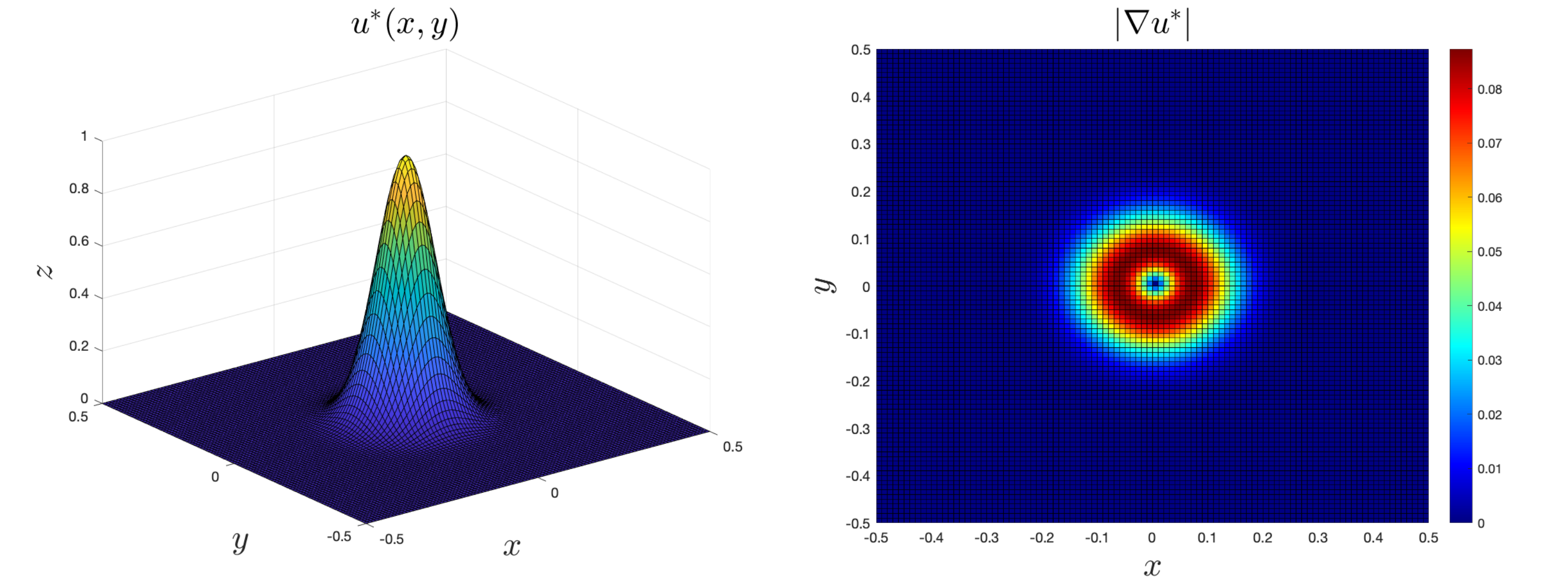
For testing purposes, we will construct the problem for a given solution:

\[ u^*(x,y)= e^{-100(x^2 + y^2)} \cos \pi x \cos \pi y \]

The gradient of this functions is

\[ \nabla u^* = \begin{bmatrix} -e^{-100(x^2 + y^2)} (200 x \cos\pi x + \pi \sin\pi x) \cos\pi y\\ -e^{-100(x^2 + y^2)} (200 y \cos\pi y + \pi \sin\pi y) \cos\pi x \end{bmatrix}, \]

see Figure 1, while the source term reads:

\[ f(x,y) = -e^{-100(x^2 + y^2)} \Bigl\{400 \pi (x \cos\pi y \sin\pi x + y \cos\pi x \sin \pi y) +2\left[20000 (x^2 + y^2) - 200 - \pi^2 \right]\cos\pi x \cos\pi y \Bigr\} \]

Figure 1: Analytical solution and the norm of its gradient

First, we will verify the implementation by running the code without the refinement loop:

./mixed_poisson -file_name test.h5m -base_order 2

Using meshes with different element sizes and setting different approximation orders, we can study the convergence of e.g. field \(u\), see Figure 2(a), which for the considered mixed formulation satisfies the following a priori error bound, see [12]

\[ ||u^h-u^*||_{\Omega}\leq C(u,\mathbf{q})\,h^{p} \]

where \(h\) is the element size, \(p\) is approximation order for fluxes field \(\mathbf{q}\) and order for field \(u\) is \((p-1)\).

Figure 2: L2 error of the numerical solution for different approximations orders with respect to (a) element size, (b) number of DOFs

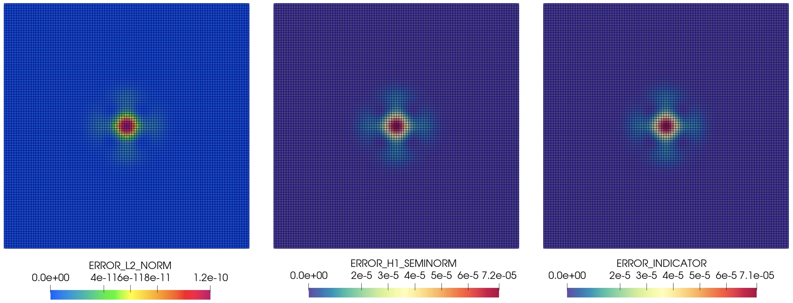
Furthermore, we can plot the values of the local errors and local error indicators \(\eta_e\), given by \eqref{eq:indic}. Figure 3 shows that the considered error indicator (difference between the gradient of field u and the flux) is very close to the H1 seminorm of the error computed using the analytical solution. Moreover, the indicator is very effective in highlighting the regions where the L2-norm of the solution is pronounced.

Figure 3: Local error and error indicator

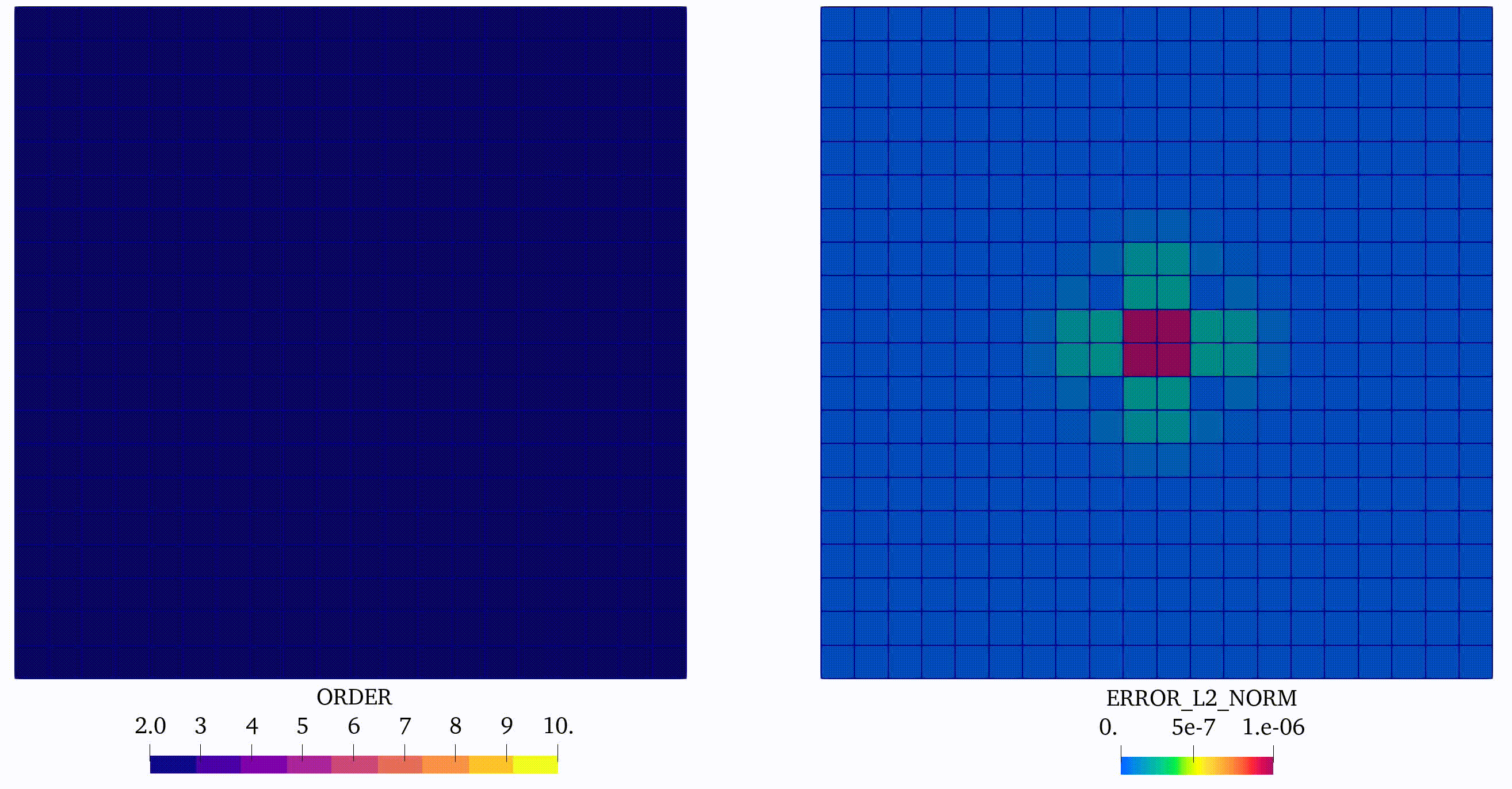
Next, we run the code invoking the adaptive p-refinement:

./mixed_poisson -file_name test.h5m -base_order 2 -ref_iter_num 10

In this case, we can observe coherent evolution of the approximation orders saved on element tags and the corresponding distribution of the error in the domain, see Figure 4:

Figure 4: Approximation order and local error for several iterations of the adaptive p-refinement

Finally we extend the convergence analysis and plot the error as a function of number of DOFs used in simulation, see Figure 2(b). We can observe in this simple example the effectiveness of using the p-adaptivity, driven by the error indicator. Indeed, such an approach, which is increasing approximation order only in regions where the error is pronounced, requires much less DOFs then the approach based on global h- or p-refinement to obtain the same accuracy of the solution.