 |
v0.14.0 |
|
v0.14.0 |
In this tutorial we will solve a simple Poisson's equation with homogeneous (uniform in space) boundary condition using MoFEM. The physical example of this equation is that you have a membrane that is fixed at its boundary and it experiences a uniformly distributed force on its surface, then you are asked to estimate the displacement of the membrane. The strong form of the problem as follows
\[ \begin{align} -\nabla \cdot \nabla u(\mathbf{x}) &= f \quad {\rm in} \quad { \Omega}, \\ { u}(\mathbf{x}) &= 0 \quad {\rm on} \quad \partial { \Omega}, \end{align} \]
where \( { \Omega} \) denotes the domain occupied by the body and \( \partial { \Omega} \) is the boundary of the domain. Additionally, \( f \) is the source function and \( {\bf x} \) is the position in 2D or 3D space of a point in the domain.
Let consdier a Poisson problem on a rectangle domain with homogenous boundary conditions and source function \( f \), the analytical solution can be found. However, as the first practice with MoFEM, we are solving it numerically using a finite element approach. This is done by subdividing the domain into multiple elements, building piece-wise approximations, and solving a discrete problem.
As you may have already learned from the basic finite element method, in order to approximate a field \( u \) of the problem equation. We need to derive the weak form it. The procedure to achieve it is as follows
\[ \begin{equation} -\int_\Omega \delta u(\nabla \cdot \nabla u ) ~d\Omega= \int_\Omega \delta u f ~d\Omega. \end{equation} \]
\[ \begin{equation} \int_\Omega \nabla \delta u \cdot \nabla u ~d\Omega - \int_{\partial \Omega} \delta u {\bf n} \cdot \nabla u ~d\partial \Omega = \int_\Omega \delta u f ~d\Omega. \end{equation} \]
It is noted that the test function \( \delta u \) has to satisfy the homogeneous boundary condition, i.e. \( \delta u=0 \) on \( \partial \Omega \). Substituting it to the above equation, we finally obtain the weak form of the problem\[ \begin{equation} \int_\Omega \nabla \delta u \cdot \nabla u ~d\Omega = \int_\Omega \delta u f ~d\Omega, \quad \forall \delta u \in H_{0}^{1}(\Omega), \end{equation} \]
where the space for test function \( \delta u \) is \( H_{0}^{1}(\Omega):=\left\{v \in H^{1}(\Omega) \mid v=0 \text { on } \partial \Omega\right\} \).We are now solving this equation of the weak form instead of the original equation. This equation is asking for the solution of \( u \) that is true for all test function \( \delta u \). In order to achieve it, we will approximate \( u \) following a process in finite element called discretisation which will be presented in the next part.
As mentioned above, instead of trying to solve the problem analytically, we will approximate \( u \) assuming its solution has the form
\[ \begin{equation} u \approx u^h = \sum_{j=0}^{N-1} \phi_j \bar{u}_j. \end{equation} \]
This expression can be interpreted as follows. Find the approximate solution \( u^h \) of \( u \) where \( u^h \) is calculated by summing the contribution of base function \( \phi_j \) with the coefficient of the contribution is \( \bar{u}_j \).
Sometimes, \( \phi_j \) is also called shape functions and \( \bar{u}_j \) called degrees of freedom (DOFs) of the problem. In the implementation process, which will be discussed later in this tutorial, MoFEM gives you values of \( \phi_j \) by default (provided that you give it some hints) and you will find the solution of \( u^h \), of course, with the help of MoFEM.
Keep in mind that, in the weak form, we have another term that also needs to be taken care of, that is the test function \( \delta u \). As we were saying, the weak form has to be satisfied with all test function \( \delta u \) meaning it has to be true with the arbitrary choice of \( \delta u_i=\phi_i \).
Substituting \( u \) and \( \delta u \) into the weak form, we have the discrete form of the problem given by
\[ \begin{equation} \int_{\Omega^e} \nabla \phi_i \cdot \nabla \left( \sum_j \bar{u}_j \phi_j \right) ~d{\Omega^e}= \int_{\Omega^e} \phi_i f ~d{\Omega^e}. \end{equation} \]
Moving \( \bar{u}_j \) outside of the parentheses and rearranging the equation, we have
\[ \begin{equation} \sum_j \left( \int_{\Omega^e} \nabla \phi_i \cdot \nabla \phi_j ~d{\Omega^e} \right) \bar{u}_j = \int_{\Omega^e} \phi_i f ~d{\Omega^e}. \end{equation} \]
Now, the problem becomes: finding the vector of coefficients (or DOFs) \( {\bf U} \) such that
\[ {\bf K u} = {\bf F}, \]
where \( {\bf K} \) and \( {\bf F} \) are the global stiffness matrix (left hand side) and global force vector (right hand side) calculated over the whole domain, respectively. \( {\bf K} \) and \( {\bf F} \) are obtained by assembling all elements (entity) in the domain, and the components of element stiffness matrix and element force vector are calculated as
\[ \begin{align} K_{ij}^e &= \int_{\Omega^e} \nabla \phi_i \cdot \nabla \phi_j ~d{\Omega^e}, \\ F_i^e &= \int_{\Omega^e} \phi_i f ~d{\Omega^e}. \end{align} \]
One thing we can notice here is that the matrix \( {\bf K} \) is symmetric which means there will be opportunity to save time later in the implementation.
We are almost at the place where we can start the implementation, but still, you may ask how computers can handle the integral terms. Of course, we will not ask computers to calculate the integrals directly in an infinite sense, instead it is done using quadrature which is in a finite sense and commonly used in finite element method. In other word, the integrals are approximated by the sum of a set of points on each element along with their weights as follows
\[ \begin{align} K_{ij}^e &= \int_{\Omega^e} \nabla \phi_i \cdot \nabla \phi_j \approx \sum_q \nabla \phi_i \left( {\bf x}_q \right) \cdot \nabla \phi_j \left( {\bf x}_q \right) W_q \left\|\mathbf{J}_{g}^{e}\right\| \label{eqn_stiffness}, \\ F_i^e &= \int_{\Omega^e} \phi_i f \approx \sum_q \phi_i \left( {\bf x}_q \right) f \left( {\bf x}_q \right) W_q \left\|\mathbf{J}_{g}^{e}\right\|, \end{align} \]
where \( {\bf x}_q \) and \( W_q \) are the location and weight of the quadrature point, respectively. Meanwhile, \( \left\|\mathbf{J}_{g}^{e}\right\| \) is the determinant of the Jacobian of the transformation of the element \( e \) from physical coordinates to parent coordinates. For triangular elements, this determinant equals to the area of the element. These equations can be interpreted as follows
The approximated value of the component at row \( i \) and column \( j \) of the element stiffness matrix \( K \) of element \( e \) is calculated by taking the summation over all quadrature points of the multiplication of
Likewise, the approximated value of the component at row \( i \) of the element force vector \( F \) of element \( e \) is calculated by taking the summation over all quadrature points of the multiplication of
More details on the numerical integration can be found at the tutorial FUN-1: Integration on finite element mesh.
To this end, we have established a linear system of the primary variable \( {\bf U} \) through \( {\bf K} \) and \( {\bf F} \). In MoFEM, we will use an iterative solver (KSP) to solve for \( {\bf U} \) and apply steps to postprocess the solution and visualise it.
An immediate question you may have regarding the implementation is how to implement the matrix \( {\bf K} \) and vector \( {\bf F} \). This is done through the implementation of the so-called User Data Operators. UDOs are the essential part of MoFEM and they are present in all finite element problems implemented in MoFEM. UDO is normally called Operator (for short) by MoFEM developers. Once UDOs are implemented, they will be pushed to the working pipeline.
Here we have introduced two important concepts in MoFEM
As a common practice, typically all the implementation of UDOs for a specific problem is put in a *.hpp file. This file will be included in the main *.cpp file which contains all the necessary classes and functions. Detailed explanation of the implementation of UDOs, how you pushed UDOs to Pipeline as well as development of classes/functions are presented below
As described previously, solving the Poisson problem with homogeneous would require the computation and assembling of the matrix \( {\bf K} \) and vector \( {\bf F} \). These essential processes of computation and assembling will be handled by two different UDOs which separately deal with the matrix and vector. They are:
Before going into details of the implementation of the two UDOs in poisson_2d_homogeneous.hpp, let's have a look at the first few lines of code file that includes some libraries for finite element implementation. The code is based on C++ libraries with advanced aliases, and declaration/initialisation. Apart from that, the dimension(2D/3D) of the problem can easily be assihned from the EXECUTABLE_DIMENSION which will discuss later.
Next, Users can also learn a general structure of any UDOs implemented in MoFEM to many extend. So, we will look in details how the following two main User Defined Operator(UDO)s of the problem can be implemented.
This UDO is responsible for the calculation and assembly of the left-hand-side matrix \( {\bf K} \)
First, let's look at the structure of this UDO to calculate matrix \( {\bf K} \).
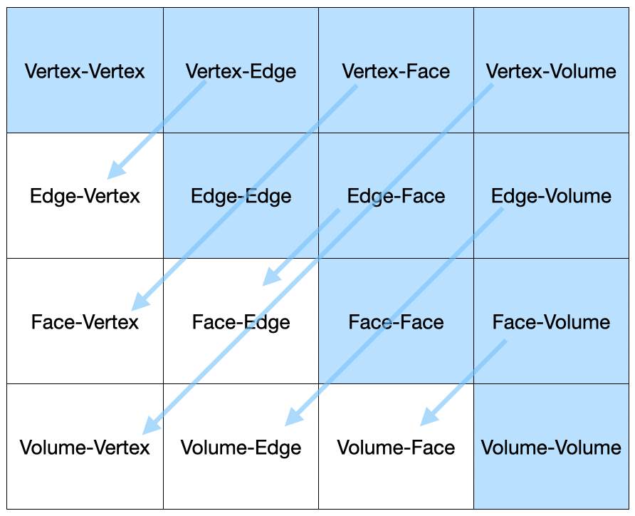
We have the class OpDomainLhsMatrixK that is inherited from AssemblyDomainEleOp which is the alias of the base chain of specialized template FormsIntegrators<DomainEleOp>::Assembly<PETSC>::OpBase. This operator also accelerate the process of assembling local matrix to global matrix. Here, the forms integrators using the DomainEleOp type is a templated parameter to assembly using the PETSc library. Here, the newly created class has two public objects OpDomainLhsMatrixK() and iNtegrate which can be accessed from outside of the class. This follows the concept of data encapsulation to hide values and objects inside the class as much as possible. We will discuss a little more details of those four objects of the class in the followings
OpDomainLhsMatrixK() iNtegrate locMat Now we take a closer look on the details of the implementation of the member function iNtegrate(). Full code for this function as follows
First, let's discuss the structure of this function
For specific tasks, the data structure is adapted based on the problem's dimension. Such as solving a 2D or 3D Poisson problem, the code can utilize different entities types e.g. edges, faces, volumes. For example, the entities or elements are provided accordingly using PipelineManager::ElementsAndOpsByDim<SPACE_DIM> which is aliased as ElementsAndOps.The DomainEle::UserDataOperator is used to assemble using the forms integrator AssemblyDomainEleOp. This can be seen in the code, particularly in the struct OpDomainLhsMatrixK. The function's parameters of iNtegrate are row_data and col_data are referencing to objects of type EntitiesFieldData::EntData. These parameters make ready the data related to degrees of freedom, basis function values, and field values for the rows and columns of the operation.
In MoFEM, functions are written with check and error handling using keywords like MoFEMErrorCode, MoFEMFunctionBegin, and MoFEMFunctionReturn(0). These indicate the execution of functions and the success or failure of the operation. These arguments are used to handle errors like try() or catch() in basic c++ systematically.
Now, moving into the main implementation of iNtegrate() function, we will see information about the number of DOFs on row and column are extracted from the database
Once the program is confident that the data for row and column are all valid, it starts to initialise the local stiffness matrix whose components will be calculated and assembled to the global matrix.
Then you will get the area for 2D or volume for 3D which is needed later when you integrate the function to calculate the stiffness matrix.
It is worth noting that getMeasure() is a generic function and the value you get depends on which entity type you are working with. For example, in this UDO, you are working with face entities (triangles), getMeasure() gives you face area. If you are dealing with edge (for boundary element) or volume entities (for volume domain), you would get edge length or element volume, respectively.
Next, as required for the calculation of stiffness matrix in Eq. (3), we need the number of integration points ( \( q \)) and their weights ( \( W_q \)) which can be done as follows
Here getFTensor0IntegrationWeight() is a function of MoFEM::ForcesAndSourcesCore::UserDataOperator and it returns a zeroth-order FTensor object (Tensor template library) that stores value of integration weight. We prefer to use FTensor anywhere we can because it is compact and highly efficient. In MoFEM implementation, FTensor object is normally named with the prefix t_.
Once the number of Gauss points and their weights are determined, the remaining component to calculate stiffness matrix would include the gradients of the basis function evaluated at the integration (Gauss) point, \( \nabla \phi_i, \nabla \phi_j \) ,for row and column, respectively, and the loop over all the Gauss points. They are done in the following part of the code
Here you can see inside the loop over the integration points, we have two other nested loops that loop over the row ( \(i\)) and column ( \(j\)) DOFs of the matrix which is ultimately calculated similarly to the way they are presented in Eq. (11)
where a is the intermediate variable of type double and calculated earlier as
where area can be considered as the determinant of the Jacobian of the transformation from the physical (global) coordinate system to the reference (local) coordinate system. See more about the integration and Jacobian at FUN-1: Integration on finite element mesh.
It should be noticed that at the end of each loop over the row and column DOFs, t_row_diff_base and t_col_diff_base which have the values of the gradients of the basis function are moved/shifted to the next chunk of the memory which stores values of another set of gradients of basis function associated with DOFs. The same technique is applied to move t_w to the weight of the next Gauss point in the memory.
Note: You might have also recognised that in the traditional finite element implementation, you will probably have, at the same place of the code, the structure of the main nested loop like this
In MoFEM's finite element implementation, there are some differences worth noting. While nested loops are still used, the implementation of the User Data Operator (UDO) involves a single loop over integration points. Within this loop, local stiffness matrix components are computed and then assembled into the global matrix. The loop over elements referred to as entities in the context of Hierarchical basis functions Details of how this loop is triggered is presented in solveSystem().
That concludes the description of the code segment responsible for calculating the components of the element stiffness matrix.
In this part, we will talk about the implementation of the second UDO Poisson2DHomogeneousOperators::OpDomainRhsVectorF which is responsible for the calculation and assemble of the right-hand-side force vector \( {\bf F} \)
Similar to what implemented for the \( {\bf K} \) matrix we discussed above, the implementation of the UDO for the \( {\bf F} \) vector has very similar structure with slightly different functions
We have the public objects of OpDomainRhsVectorF() and iNtegrate() and private object of locF. Here the name of the main function is changed to OpDomainRhsVectorF to reflect what it does. Additionally, as we are calculating and assembling vector instead of matrix, we need only one input of field_name and we tell MoFEM that we are doing the operation of row for the vector by specifying DomainEleOp::OPROW. Similarly for function iNtegrate(), it requires all three groups of the input but only one for each group instead of two as we had for the stiffness matrix.
The implementation of this essential function of iNtegrate() for force vector calculation and assembling also has very similar structure to its matrix UDO counterpart. The code for this function is as follows
A part from the input arguments of this function is slightly different from the UDO for stiffness matrix. In this UDO for force vector, we use the base function value to calculate the components of local vector reflecting what is presented in Eq. (4) and only need to loop over row DOFs as follows
and later using the constant body source (force) that is predefined at the beginning of the *.hpp to calculate the local vector
That is all for the implementation of UDOs that are responsible for the calculation and assembling of the LHS matrix \( {\bf K} \) and RHS vector \( {\bf F} \). Having the essential components implemented, you now may ask how those UDOs are called in the main program. This is done through the process called push operator to the Pipeline and you will find out in more details later in this tutorial, assembleSystem().
Next, we will look in detail how the main program, including class and functions, is implemented.
This main class Poisson2DHomogeneous contains functions and each of which is responsible for a certain task of a finite element program. Intially, the field name has named as "U" string to recognsie it well. Next the EXECUTABLE_DIMENSION is the considered for the dimension of the mesh. To generalize, the value is assined to the Space dimension of problem.
The public part of the class includes a constructor and function runProgram() that calls other functions to perform finite element analysis.
Then there are private functions doing certain tasks and can be recognised by their names
It is followed by the declaration of member variables that will be used in one or some of the member functions declared above
Now is the constructor
The constructor specifies
mField(m_field): The MoFEM instance that is the backbone of the programNow the first function that actually does some finite element task is the function responsible for reading input mesh
Apart from the codes for error handling, the main three lines of code is a standard way to read an input mesh using Simple interface. Interface in MoFEM is a set of rules through which program developers use to setup a problem. Simple interface provides simplest but also less flexible way to setup a problem. More on the interfaces can be found at MoFEM interfaces. Implementation of more advanced interfaces will be presented in later tutorials.
Next is the function that is responsible for setting up the finite element problem
This function has
simpleInterface->addDomainField: It is important to understand that we need to add the domain field through the simpleInterface only as the field at the boundary is zero (homogeneous) for this particular example hence no need to add the boundary field. The addition of the domain field requires the followingsH1 - scalar space) - function space can also be H(curl), H(div), L2 depending on physical properties of the field you are approximating, see more at FieldSpaceAINSWORTH_BERNSTEIN_BEZIER_BASE) - base can also be AINSWORTH_LEGENDRE_BASE, AINSWORTH_LOBATTO_BASE, DEMKOWICZ_JACOBI_BASE , see more at FieldApproximationBase, and1) as the current problem is a scalar-field problem. This will be 3 for vector-field problem.simpleInterface->setFieldOrder: Set the polynomial order of the approximation of the fieldsimpleInterface->setUp(): Finally, do the setup of the problem.This function deals the boundary condition and its implementation for the current problem is as follows
To ensure the code reads the boundary conditions, it's essential to generate the mesh that includes the required attributes or values. Specifically, blocks in the mesh must be labelled with the name "BOUNDARY_CONDITION". In other cases where multiple boundary conditions are involved, you should assign distinct names using numbers, such as "BOUNDARY_CONDITION_1", "BOUNDARY_CONDITION_2", "BOUNDARY_CONDITION_3", and so on. This naming scheme helps in distinguishing and applying different boundary conditions to their respective blocks within the mesh.
Though the application procedure is pretty straightforward but the underlying process of applying these boundary conditions is not immediately obvious. Users can jump to the next section without understanding the underlying process of it.
If we consider \( {\bf u} \) as the solution vector such that \( {u} = [u_1, u_2, u_3, u_4, \ldots, u_n] \), we will essentially eliminate the DoFs associated with entities that are part of the "BOUNDARY_CONDITION" blocksets. In this context, let's say the \( \bf{u_0} \) represents the vector after removing the DOF from BC. For example, \( {u_0} = [u_1, u_2, u_3,.. .. u_\text{n-m}, 0 ,0\ldots, 0] \). However, we need to reintroduce these removed DoFs later on to make the solution admissible for the boundary values as well. To accomplish this, we will incorporate an additional vector \( {\bf u^e} \) with the current \( {\bf u_0} \), as in (14).
\[ \begin{equation} \bf {Ku}= f \end{equation} \]
\[ \begin{equation} \bf {K(u_0 + u_e)}= f \end{equation} \]
Here, \( u_e \) is the vector where we will impose those removed degrees of freedom in it. For example,
\[ \begin{equation} {\mathbf { u}_e} = \left[ \begin{array}{cccc} {0} & {0} & {0} & \ldots & {u_\text{n-m+1} } & {u_\text{n} } & \end{array} \right] \label{eq:u_e} \end{equation} \]
Here, \( u_\text{n-m+1} \) and \(u_\text{n} \) denotes DOFs the of BOUNDARY_CONDITION Blockset.
This approach will allow us to streamline the procedure and ensure that the removed degrees of freedom are properly reintegrated into the calculations. However, to simplify this cumulative process, we will address rest of the part during the assembling phase in the upcoming sub-section.
This part is about the function that is responsible for the assembling of the system of equations. In between, we will also go through the code for setting the DOFs to the BC.
At the beginning of the section assembleSystem(), recall the two important concepts in MoFEM, namely UDO and Pipeline. While how the implementation of UDOs has been shown in User Data Operators, here you will see how the implemented UDOs are pushed to the Pipeline.
Apart from pushing UDOs to the main program, assembleSystem() ()function is mainly responsible for setting operators implementing to the pipelines for KSP solver (iterative linear solver provided by PETSc). The full source code for the function is as follows:
pipeline_mng) that manages two main pipelines which are:getOpDomainLhsPipeline: responsible for calculations of the left hand side matrixgetOpDomainRhsPipeline: responsible for calculations of the right hand side vector OpDomainLhsMatrixK is pushed to the LhsPipeline. boundaryCondition(), we modified \( \bf{u} \) and we were waiting to impose the removed DoFs to get the admissible solution. Here, this operation is done by the lamda function 'set_values_to_bc_dofs'.We enforce the following code snippet to set dofs. First we get the reference \( \bf{u}\) for BC. Then using 'get_bc_hook' as preprocessing of object 'fe' we set the boundary condition values to \( \bf{u_e} \).
Note:For the current homogenous problem, if we consider zero boundary condition, that endsup with all the values of \( \bf {u_e} \) as zero. So then the remainings from the equation (15) is \( \bf {K u_0} = \bf {f}\). However, in case of non-zero BCs we have to consider \(\bf {K u_e}\) in the next part.
So the rest of the code should be organised as follows:
Here, the lamda function calculate_residual_from_set_values_on_bc is to get the \(\bf {K{u_e}}\). Inside of it, the OpInternal integrator serves a dual purpose: it undertakes system of equations and assembles the matrices, effectively performing a linear multiplication. Upon pushing OpInternal to the pipeline manager, -1 is passed as it is alongside \( \bf K {u_e} \) as in equation (17).
\[ \begin{equation} \bf {K u_0} = f - \bf {K u_e} \end{equation} \]
We do not need derivative of the approximation function to calculate force vector in UDO OpDomainRhsVectorF. Consequently, the operators for recalculating inverse of Jacobian is not needed as well as it is integrated with MoFEM.
This function is responsible for setting the Gauss integration rules and it looks like this
Here \( p \) is the polynomial order of the approximation function. For the LHS matrix, we are calculating the integral of function \(\nabla \phi_i \cdot \nabla \phi_j\) so the polynomial order of the integral is \( p - 1 \) plus \( p - 1 \) resulting \( 2 * (p - 1)\) as we see in the implementation of the integration rules for the LHS. Similarly, as we calculate the integral of \( \phi_i\) for the RHS, we use \( p \) as the integration rule of the RHS. Having the integration rules, MoFEM will automatically determine the number of integration (Gauss) points that need to be used for each entity (element). Here you can see MoFEM allows you to choose different integration rules for different operators.
Having the computation of LHS and RHS is defined in the previous function. We now can actually solve the system of equations using iterative KSP solver from PETSc.
The codes for the function that is responsible for solving the systems of equations look like this
It starts first with getting the pipeline manager
Then create the KSP solver using wrapped function in MoFEM (pipeline_mng->createKSP()) and setup the solver using PETSc functions
Next is getting the Discrete Manager (dm) which is a common object allowing things implemented in MoFEM talk to things implemented in PETSc before initilising the RHS and solution vectors
At this particular point, Discrete Manager allows the two pipelines (responsible for LHS and RHS) implemented in MoFEM to be used as the input for KSP solver implemented in PETSc. From that, the solution vector \( {\bf U} \) of the system of equations \({\bf KU=F} \) will be obtained when the KSP solver is triggered by this
It is important to note that all the implementation of the UDOs presented in the previous sections was just the definition. All the calculations (all the loops to calculate matrix and vector entries implemented in UDOs) are only triggered when the line of code above calling KSPSolve() function is executed.
Lastly, the results are scattered through DM and ready to be fed to the output mesh in the next step
This function is solely responsible for the postprocessing of the results writing the calculated field values to the output mesh.
Finally, having all the necessary tasks implemented in the corresponding functions, we can now put them together in the last function of the main class. This function is responsible for the calling sequence which is similar to most of other finite element programs
This main() function does not do much job apart from creating the top-level class and call the function to trigger the analysis
So you can see, at the beginning, it creates the Discrete Managers that enable information flows between MoFEM (finite element implementation), MOAB (element topology management), and PETSc (algebraic solvers). After that, it creates variable poisson_problem of type/class Poisson2DHomogeneous which is previously defined and then run the analysis by triggering the public function runProgram().
In order to run the program that we have been discussing in this tutorial, you will do the following steps
poisson_2d_homogeneous is located. Depending on how you install MoFEM shown in this page Installation with Spack (Scripts), going to the directory would be something similar to thisOnce the analaysis is complete, you see all output messages printed to the terminal
Then, you also see in the directory where you run the analysis, it now has the newly created output file, namely out_result.h5m. The output can be visualised in a visualisation software. If you would like to open the output in the free software of Paraview, you would need to convert the input file to *.vtk format by running the following command line in your terminal
Then open it in Paraview and use the filter WarpByScalar, you will be able to see the deformation as below
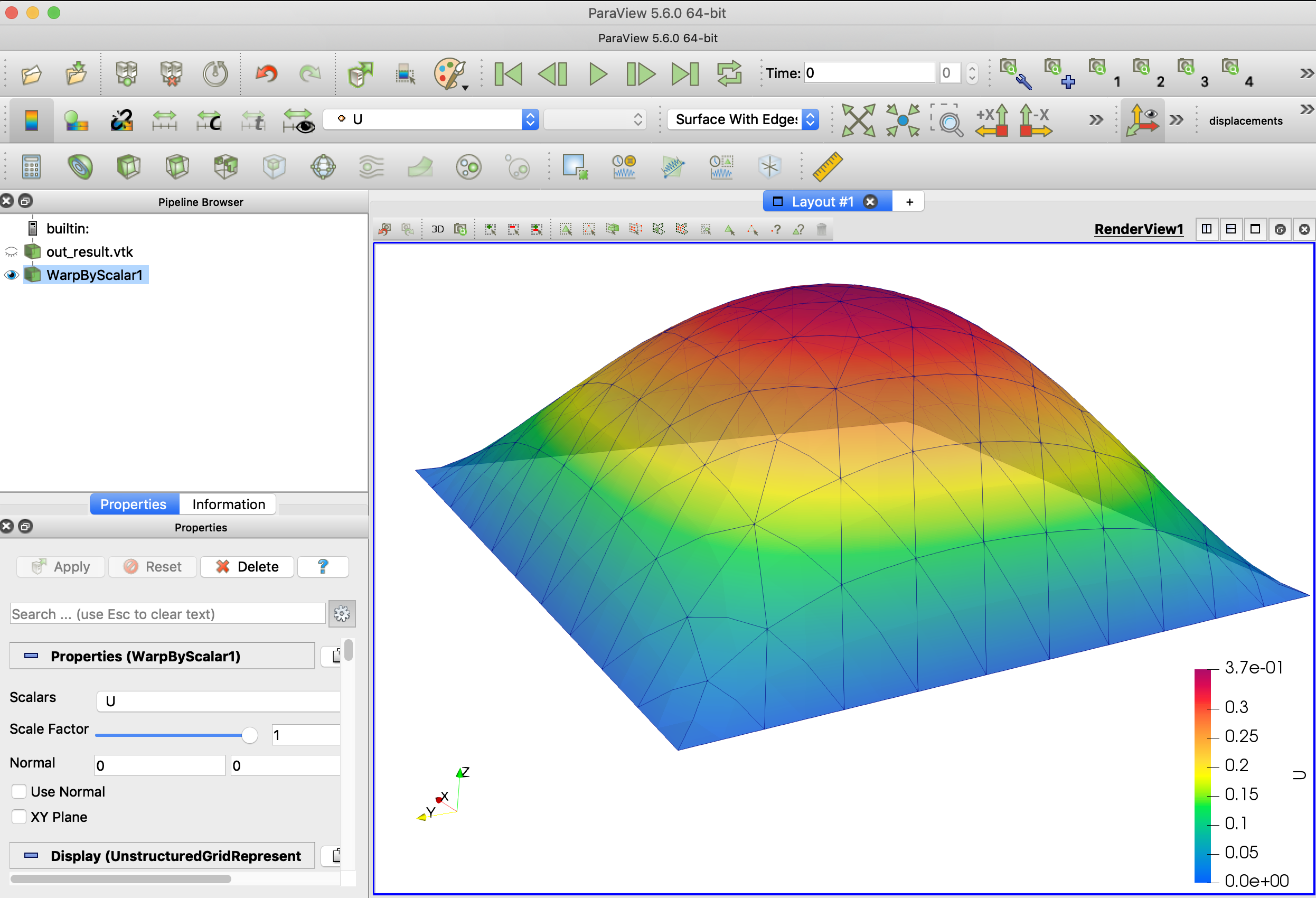
As mentioned at the beginning of this tutorial, this Poisson equation with homogeneous boundary condition helps to predict the deformation of a membrane that is fixed at the boundary bearing an uniformly distributed force on its surface. In this case, the force \( f=5.0\) is hardcoded in the code.
You can test yourself how the increase/decrease in approximation order affects the number of DOFs and the analysis time. Also, you can do the same investigation but by changing the mesh density.
Regarding the implementation in MoFEM, it is important that you get the concept of developing/using UDOs to evaluate the matrices and vectors and then push them, in a certain order, to the Pipelines where calculations are done sequentially. These concepts will apply to all of the programs implemented in MoFEM.
You can find the complete code to solve 3D version of the Poisson problem with homogeneous boundary condition, using the same source code by setting variable EXECUTABLE_DIMENSION=3, see CMakeList.txt file in mofem_install/um_view/tutorials/scl-1/
To run the analysis, you will follow very similar procedure as for the 2D case using the same param_file.petsc file with slight changes in the command lines
The plain program for both the implementation of the UDOs (*.hpp) and the main program (*.cpp) are as follows
