 |
v0.14.0 |
|
v0.14.0 |
The first lesson is solely devoted to numerical integration. Integration is essential for most of the numerical methods (except for the collocation method) used to solve partial differential equations (PDEs).
The most straightforward interpretation of the finite element method is to consider it as a method for integration of functions on complex shapes. The integration domain is divided into elements with primitive shapes, e.g. edge, triangle, quad, tetrahedron, or hexahedron, and on each element integration rule for the primitive shape is evaluated. Thus a complex problem is broken into many simple elements, on which the same simple procedure is executed over and over. Such repeatable tasks make it a perfect method for a computer.
We will present the problem of numerical integration by calculating moments of inertia. Moments of inertia characterise the distribution and amount of the mass in the body and have various engineering applications.
First, we explain essential formulas and provide a definition of moments of inertia. Next section is dedicated to the theory, and finally we show details of implementation in MoFEM.
For future references we provide a table of some essential mathematical notations which will be used in this and following lessons:
| Subscripts (lower indices) and superscripts (upper indices) | Font style | ||
|---|---|---|---|
| normal | bold | normal with overline (bar) | |
| without sub- or superscript | scalar (0-rank tensor) e.g. \(\rho, M, v, a, \ell\) | higher-rank (1,2, ...) tensor e.g. \(\mathbf{x}, \boldsymbol{\xi}, \boldsymbol{\lambda}, \mathbf{S}, \mathbf{I}, \mathbf{J}\) | coefficients vector e.g. \(\bar{x}, \bar{\rho}\) |
| with subscript (lower index) | scalar value at a point e.g. \(W_g, w_g, \rho_g \) | tensor value at a point e.g. \(\mathbf{x}_i, \boldsymbol{\xi}_g, \mathbf{J}_g, \boldsymbol{\lambda}_i\) | element of a coefficients vector e.g. \(\bar{\rho}_m\) |
| with superscript (upper), except \((.)^e\) and \((.)^h\) | component of a tensor e.g. \(x^i, S^i, I^{ij}, \xi^i, \lambda^i, J^{ij}\) | coordinate basis vector e.g. \(\mathbf{x}^i, \boldsymbol{\xi}^i\) | spatial component of an element of a coefficients vector, e.g. \(\bar{x}_m^i\) |
| with superscript \((.)^e\) | corresponding to \(e\)-th element e.g. \(\rho_g^e, \mathbf{J}_g^e, \mathcal{T}^e\) | ||
| with superscript \((.)^h\) | reference to the approximation e.g. \(\Omega^h, \rho^h, \rho_g^h, \mathbf{x}^h, \mathbf{x}_g^h\) | not used | |
Numerical integration of a function \(\rho(x)\) by the means of the finite element method is given by the following general formula:
\[ \begin{align} \label{eq:num_int} I(\rho) = \int_\Omega \rho\,\textrm{d}\Omega \approx \sum_{e=0}^{N-1} \sum_{g=0}^{G-1} W_g\|\mathbf{J}_g^e\|\rho^e_g \end{align} \]
where \(W_g\) is the weight of the \(g\)-th integration point, \(\|\mathbf{J}_g^e\|\) is the determinant of the Jacobian of the \(e\)-th element's transformation from the physical (global) coordinate system to the reference (local) coordinate system (evaluated at the \(g\)-th integration point), and \(\rho^e_g\) is the value of the function at \(g\)-th integration point. Finally, \(G\) is the number of integration points per each element, and \(N\) is the total number of elements in a mesh. Typically, the sum of integration weights in each element equals to unity:
\[ \begin{align} \sum_{g=0}^{G-1} W_g = 1. \end{align} \]
Furthermore, for the case of simplexes the numerical integration formula \eqref{eq:num_int} takes a more straightforward form:
\[ \begin{align} I(\rho) \approx \sum_{e=0}^{N-1} \sum_{g=0}^{G-1} (W_g v) \, \rho^e_g, \end{align} \]
where \(v\) is the volume of an element (tetrahedron);\[ \begin{align} I(\rho) \approx \sum_{e=0}^{N-1} \sum_{g=0}^{G-1} (W_g a) \, \rho^e_g, \end{align} \]
where \(a\) is the area of an element (triangle);\[ \begin{align} I(\rho) \approx \sum_{e=0}^{N-1} \sum_{g=0}^{G-1} (W_g \ell) \, \rho^e_g, \end{align} \]
where \(\ell\) is the length of a line element (edge).In the following sections we explain how the above sums are evaluated and give additional details about the Jacobian.
The distribution of mass in the body can be characterised by moments of inertia. Moments of inertia have practical applications, they are used for analysis of motion of rigid bodies, or to characterise cross-section area in the structural analysis.
In general, moments of inertia are tensors. Zero moment is represented by a single scalar coefficient, first moment is a 1D array, i.e. a vector of coefficients, and second moment is a second-order tensor, coefficients of which for convenience can be organised in a 2D table, i.e. a matrix. Note that these coefficients depend on the observer, i.e. coordinate system, and the tensorial transformation rule describes how coefficients of moments of inertia change with the observer.
\[ \begin{align} M := \int_\Omega \rho(\mathbf{x}) \, \textrm{d}\Omega, \end{align} \]
where \(\rho\) is the material density, and \(\Omega\) is the body domain. Mass characterises how much force is to be applied for a desired body acceleration \(\mathbf{a}=\{a^i\}\) as stated by the Newton's law:\[ \begin{align} a^i = M f^i, \end{align} \]
where \(\mathbf{f}=\{f^i\}\) is the force. Moreover, the kinematic energy can be expressed as:\[ \begin{align} E_k = \frac{v^i M v^i}{2}, \end{align} \]
where \(\mathbf{v}=\{v^i\}\) is the velocity, and the summation over repeating indices is assumed. Note also, that for the zero moment the tensorial transformation rule is straightforward: the mass of an object cannot be changed by looking at it from different points and angles, so it is the same in every coordinate system.\[ \begin{align} S^i := \int_\Omega \rho(\mathbf{x}) \, x^i \textrm{d}\Omega \end{align} \]
where \(x^i\) is the coordinate in the \(i\)-th direction. According to that, the center of gravity of the body can be calculated as:\[ \begin{align} x_c^i = \frac{S^i}{M}, \end{align} \]
where \(\mathbf{x}_c=\{x_c^i\}\) are the coordinates of the centre of gravity of the body, or system of bodies. Note that if the origin is placed at the centre of gravity, then the first moment of inertia is zero.\[ \begin{align} I^{ij} := \int_\Omega \rho(\mathbf{x}) \left(x^ix^j\right) \textrm{d}\Omega, \end{align} \]
where the term \((x^ix^j)\) represents the Outer product. Second moment of inertia, analogously to mass, characterises how much torque is to be applied at the origin for desired body angular acceleration \(\boldsymbol\alpha=\{\alpha^i\}\), as follows:\[ \begin{align} \alpha^i = I^{ij} \tau^j = I^{ij} (\varepsilon^{jmn} x^m f^n) \end{align} \]
where \(\boldsymbol\tau=\{\tau^j\}\) is the torque vector, and \(\varepsilon^{jmn}\) is the Levi-Civita symbol, while the term in brackets is the cross product of the force vector and arm on which this force acts. Finally, the kinematic energy of the rotating body can be computed as\[ \begin{align} E_k = \frac{\omega^i I^{ij} \omega^j}{2}. \end{align} \]
This section is not essential and can be skipped, you may move to implementation and come back later for a more in-depth understanding of the problem.
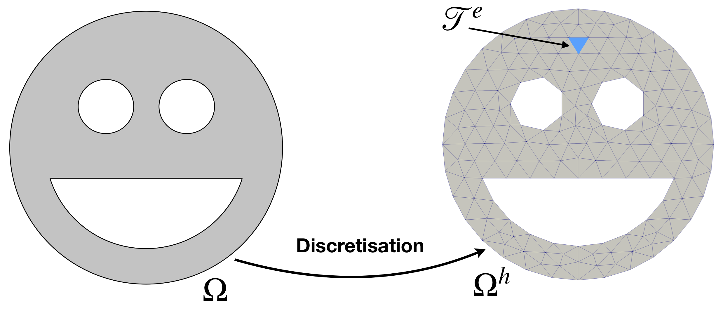
We start by dividing the integration domain \(\Omega\) into a union of non-overlapping primitive shapes (elements) \(\mathcal{T}^e\) such that:
\[ \begin{align} \bigcup_{e=0}^{N-1}\mathcal{T}^e=\Omega^h, \end{align} \]
where \(\Omega^h\) is termed as the discretisation (approximation) of the domain \(\Omega\), see Figure 1. For the rest of the tutorials, we will be using \((\cdot)^h\) to indicate a reference of the given quantity the approximation. Note that subscript h historically refers to the lateral size of an element, e.g. maximal edge length.
The integral of function the \(\rho(\mathbf{x})\), where coordinates \(\mathbf{x}\in \Omega\), can be computed approximately as a sum of integrals over all elements:
\[ \begin{align} I(\rho) = \int_\Omega \rho(\mathbf{x}) \textrm{d}\Omega \approx \int_{\Omega^h} \rho(\mathbf{x}) \textrm{d}\Omega = \sum_{e=0}^{N-1} \int_{\mathcal{T}^e} \rho(\mathbf{x}) \textrm{d}\Omega = \sum_{e=0}^{N-1} I_{\mathcal{T}^e}, \end{align} \]
where \(I_{\mathcal{T}^e}\) is the integral over the element \(\mathcal{T}^e\). The error in this computation is introduced by substituting the integration domain \(\Omega\) by a discrete mesh \(\Omega^h\). Taking a closer look at the domain \(\Omega\) in Figure 1, you can see that geometry is complex and contains curved edges. In the discretised domain \(\Omega^h\) these edges are not represented precisely, since finite elements have straight edges, thus there is some difference between the mathematical model and its finite element discretisation. However, it is good news that the error, i.e. difference between the mathematical model and its discretised version, can be controlled. You can refine the mesh until error becomes small enough, as small as you need. From the other hand, if the surfaces of the domain \(\Omega\) are flat, i.e. edges are straight, then the geometry is approximated exactly. At the same time, one can also generalise and describe edges of elements by polynomials of second and higher orders, which enables even more control of the geometrical error. However, in this tutorial, we restrict ourselves to representing the geometry by linear shape functions.
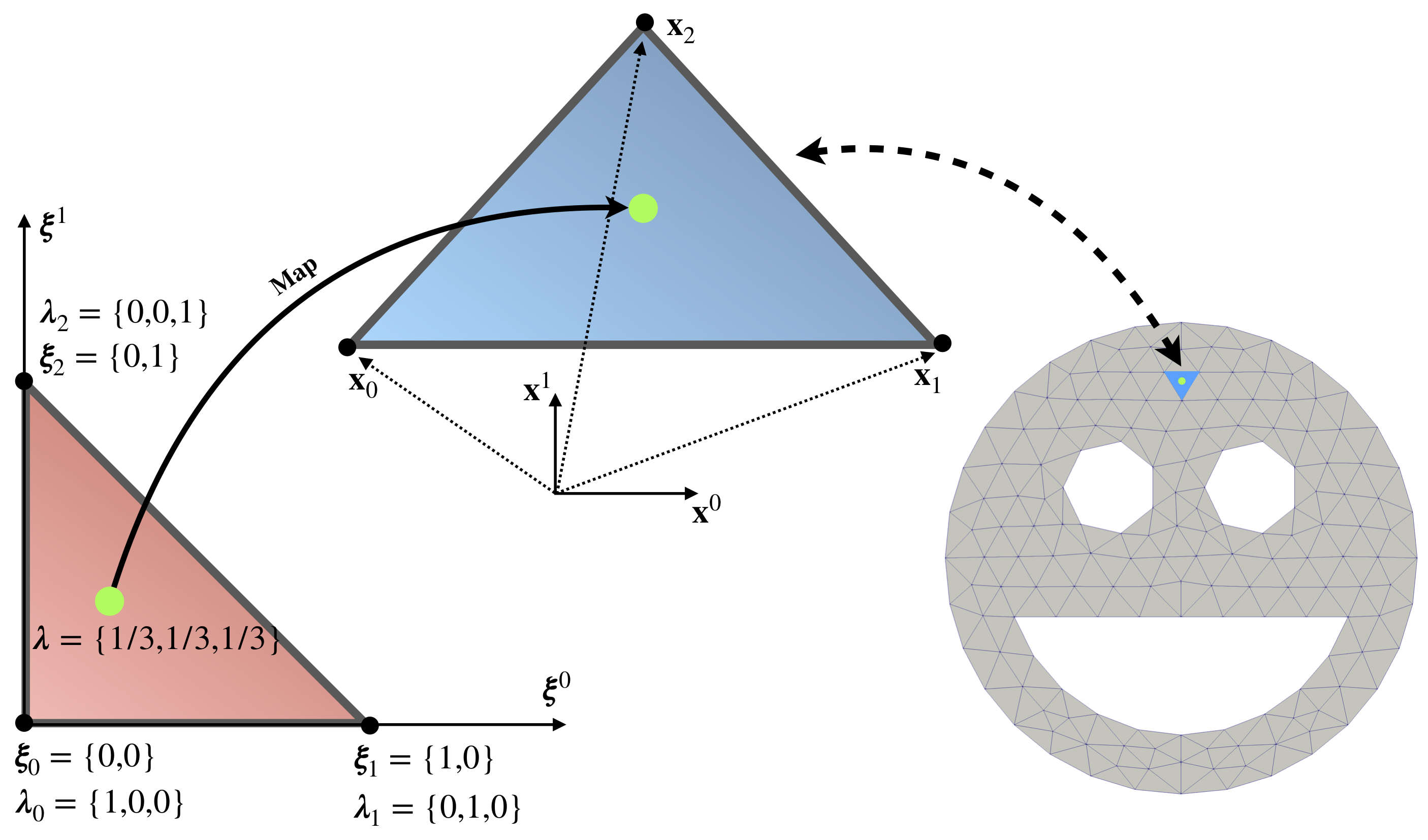
Next we discuss how the integral over a single element \(\mathcal{T}^e\) is computed. The repeated task of integrating over elements can be simplified if we perform the change of coordinates for each element from the physical (global) coordinate system \(\{\mathbf{x}^0, \mathbf{x}^1, \mathbf{x}^2\}\) to a reference (local) coordinate system \(\{\boldsymbol{\xi}^0, \boldsymbol{\xi}^1, \boldsymbol{\xi}^2\}\). Thus, the integration can be performed on a reference element which will be the same for all physical elements, see Figure 2.
For example, for a triangle element after such change of coordinates the integral can be computed as:
\[ \begin{align} I_\mathcal{T} = \int_{\mathcal{T}} \rho(\mathbf{x})\, \textrm{d}x = \int\limits_{0}^{1}\int\limits_{0}^{1-\xi^0} \rho(\mathbf{x}(\boldsymbol{\xi})) \|\mathbf{J}\|\, \textrm{d}\xi^0\textrm{d}\xi^1, \end{align} \]
where \(\mathbf{J}\) is the Jacobian of transformation of coordinates.
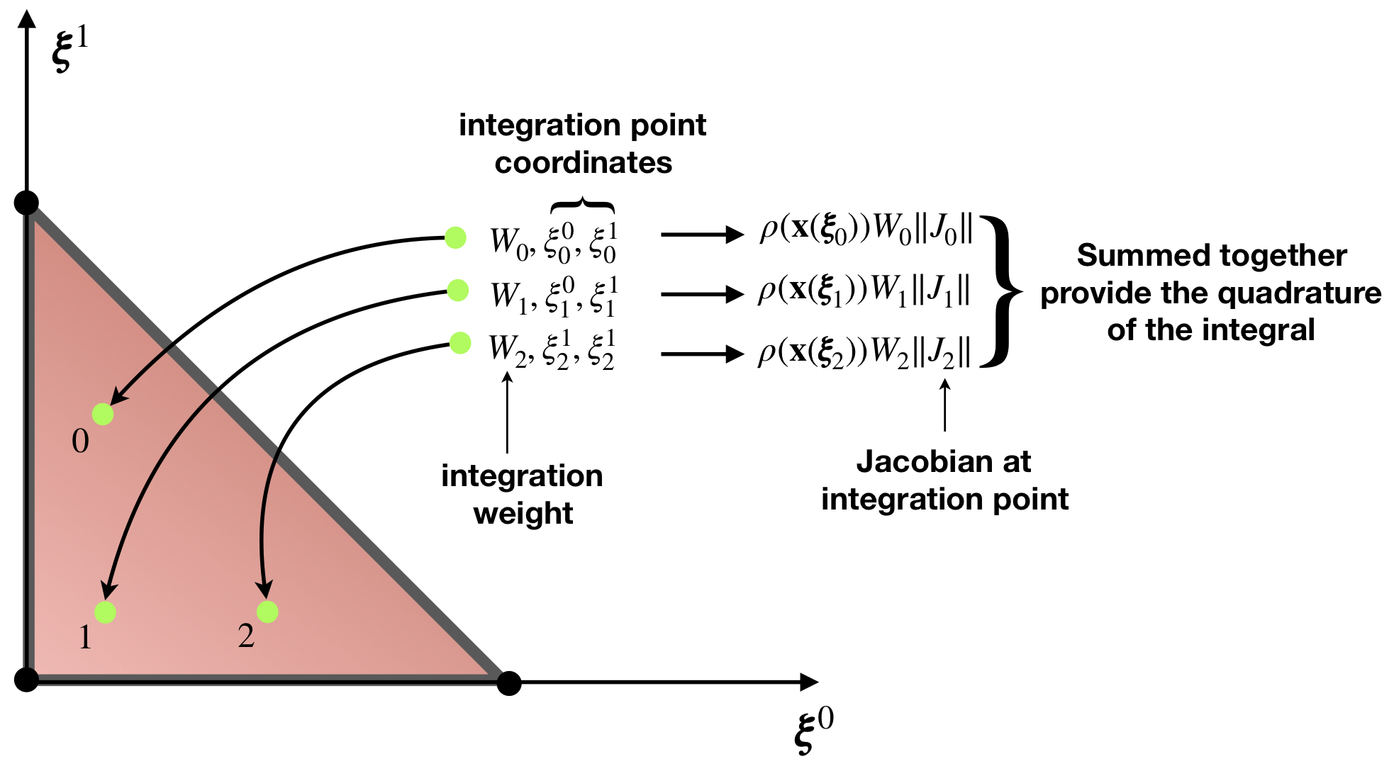
The integral \(I_\mathcal{T}\) is not to be computed analytically. Since the function \(\rho(\mathbf{x})\) in general can be arbitrary, numerical integration is used, in particular the Gauss quadrature rule is the most popular for the finite-element method. This approach requires evaluation of the integrated function \(\rho(\mathbf{x})\) at so-called integration (Gauss) points, locations of which are pre-defined for the reference element, see Figure 3.
Integration on each element, applying integration formulae, is as follows:
\[ \begin{align} I_\mathcal{T} = \int_{\mathcal{T}} \rho(\mathbf{x}) \textrm{d}\mathcal{T} \approx \sum_{g=0}^{G-1} W_g \rho\left(\mathbf{x}(\pmb\xi_g)\right) \|\mathbf{J}_g\|, \end{align} \]
where \(\rho\left(\mathbf{x}(\pmb\xi_g)\right)\) is the value of the function at \(g\)-th integration point, \(W_g\) is the integration weight of this point and \(\mathbf{J}_g\) is the value of the Jacobian at the same integration point. Note that for brevity we will also use a notation \(w_g=\| \mathbf{J}_g \| W_g\). You can see that integral is expressed simply as the sum of function values at integration multiplied by weights, something which can be easily implemented as a computer program, see also Figure 3. For a given Gauss quadrature formula polynomials can be calculated exactly up to order of integration rule \(r\), without any numerical error. Therefore, the only error of integration comes from the fact that integrated function is approximated by polynomials, i.e. \(\rho_g \approx \rho_g^h\). If the function is analytical (i.e. differentiable infinite number of times), the order of error is of \(O(h^r)\), where \(h\) is the size of the element. We will discuss how to choose the integration rule on an element in the following section.
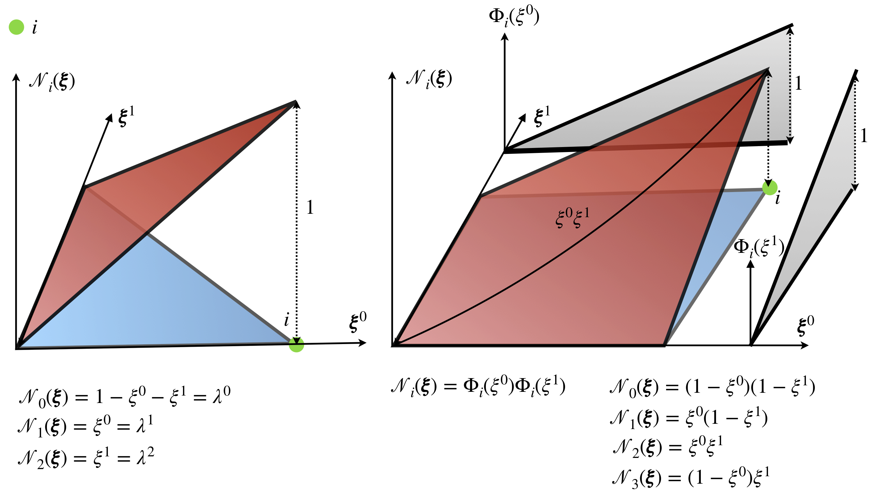
For integration on simplexes, i.e. (vertices), edges, triangles, tetrahedra, for convenience and efficiency integration points are often given by barycentric coordinates \(\pmb\lambda\), see Figure 2. For quadrilaterals and hexahedra, quadrature points are constructed by the tensor product of integration rules in 1D, see right of Figure 4. In the same way one can construct integration for other elements shapes, e.g. for prisms by the tensor product of integration on triangle and edge. For some element shapes like for the wedge, one can use Duffy transform. Duffy integration is constructed from hexahedron integration rule, and subsequently some of the nodes are collapsed. Such procedure degenerates a hexahedron to a wedge, in other words, the reference element is a hexahedron, but the physical element is a wedge.
Finally, in the example code below we will use the integration rule from the shelf. Moreover, at the moment, no matter what is the shape of a finite element, or how integration points and weights are calculated. We have to remember the numerical integration will be the sum of integration weights multiplied by function values at integration points, and we are using that in this lesson. Implementation of such integration is trivial with the use of a single loop.
The remaining question is how to evaluate field \(\rho(\mathbf{x}(\pmb\xi_g))\) at integration points? In real-world problems the data such as the density field is not given by an analytical function, but is rather known from another simulation or an experiment only at nodes of the finite-element mesh. Therefore, to make our code more general, we will compute the values of the density field at integration points using the following interpolation:
\[ \begin{align} \label{eq:interp_rho} \rho_g = \rho(\mathbf{x}(\pmb\xi_g)) \approx \rho^h_g = \sum_{m=0}^{M-1} \mathcal{N}_m(\pmb\xi_g) \bar{\rho}_m \end{align} \]
where \(\rho^h_g\) is the interpolated value at integration point \(\pmb\xi_g\), \(\mathcal{N}_m\) is shape function at node \(m\), \(M\) is the number of nodes in the element, see Figure 4, and \(\bar{\rho}_m\) is the value of the density field at node \(m\). Note that the same shape functions are used here for approximation of the geometry and for approximation of a field, this approach is known as the isoparametric finite element method. For linear shape functions, as in Figure 4, approximation error is order of \(O(h^2)\), where \(h\) is size of element (e.g. maximal length of an edge). The symbol big \(O\) is a mathematical notation which describes in this case how the error changes with the mesh size \(h\). In this particular case, it means that for every reduction of mesh size by ten times, approximation error reduces one hundred times. By making mesh smaller, the error of approximation can be controlled to achieve desired accuracy. Another way to improve the quality of the approximation and achieve arbitrary error order, is to use higher-order polynomials to approximate function \(\rho\), see FUN-2: Hierarchical approximation for more details. Note that for a polynomial of order \(p\) the approximation error is of order \(O(h^{p+1})\).
Here we present more details regarding the transformation between the physical and reference coordinate systems, while the next section is devoted to computation of the Jacobian.
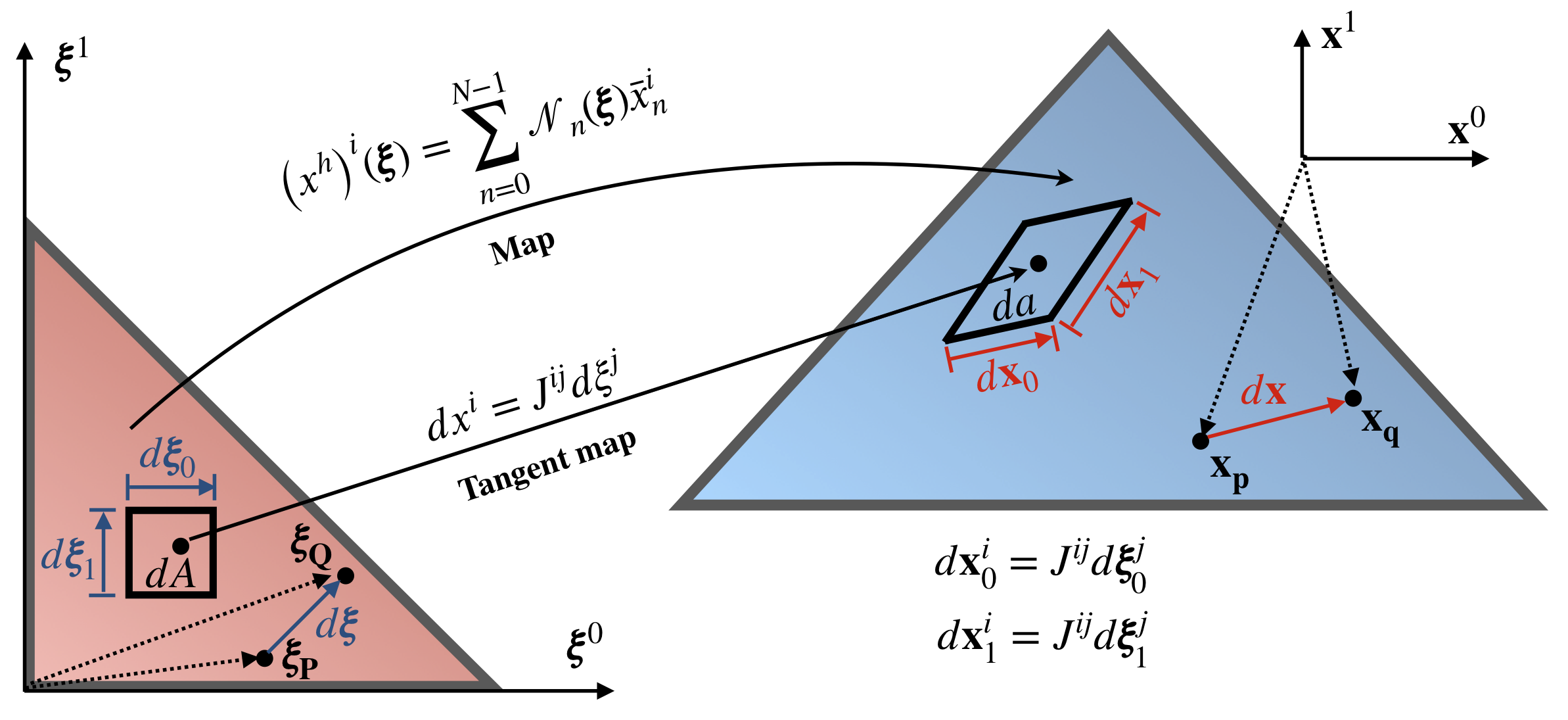
Figure 5 presents a map between the reference element (red triangle) and element in physical configuration (blue triangle). Maps transform, shift, rotate and stretch element, and establish one to one relation (at least for all points without element boundary) between coordinates in reference element \(\pmb\xi\) and physical coordinates \(\mathbf{x}\) as follows:
\[ \begin{align} \label{eq:interp_coord} \left(x^h\right)^i (\pmb\xi) = \sum_{m=0}^{M-1} \mathcal{N}_m(\pmb\xi) \bar{x}_m^i \end{align} \]
Equation \eqref{eq:interp_coord} is not very different from equation \eqref{eq:interp_rho}, the only difference is that is evaluated for every coefficient \(i=0..(d-1)\), where \(d\) is the dimension of the problem, e.g. for 3D problem \(d=3\).
Note that integration over the physical element is problematic; it is much easier to construct integration rule on the reference element and integrate on it. This way weights and integration point coordinates can be pre-calculated and stored in the table to be used for all elements on the mesh. To change the integration domain from physical element to the reference element, the concepts of a map, the tangent map and Jacobian are needed.
From Figure 5 we can see that an infinitesimal element in the reference configuration can be mapped to an infinitesimal element in the physical space by mapping infinitesimal vectors \(\textrm{d}\pmb\xi\) into \(\textrm{d}\mathbf{x}\). Expanding such map at any point \(\mathbf{q}\) into Taylor series, we get:
\[ \begin{align} x_\mathbf{q}^i = x_\mathbf{p}^i + \textrm{d}x^i = x_\mathbf{p}^i + J^{ij}(\xi_\mathbf{P}) \textrm{d}\xi^j + O\left(\|\textrm{d}\xi\|^2\right), \end{align} \]
where Jacobian is
\[ \begin{align} J^{ij}(\pmb\xi_\mathbf{P}) = \sum_{m=0}^{M-1} \left. \frac{\partial \mathcal{N}_m}{\partial \xi^j} \right|_\mathbf{P} \bar{x}_m^i \end{align} \]
Therefore, the infinitesimal vector \(\textrm{d}\mathbf{x}\) can be computed as:
\[ \begin{align} \textrm{d}x^i = J^{ij}(\xi_\mathbf{P}) \textrm{d}\xi^j, \end{align} \]
omitting higher-order terms on the right-hand side, since we focus our attention on infinitesimal elements in reference and physical configurations, and, consequently, it can be assumed that \(\|\textrm{d}\pmb\xi\|^2 = 0\) without making any error. Note that once the higher-order terms are omitted, equation mapping domain in the vicinity of a point in the reference element into the domain in the vicinity of a point in the physical element is linear. This is called the tangent map since it is accurate only in the vicinity of the tangent point. Like a tangent plane pinned to the earth, glob can represent distances accurately between locations only in the small range from where it is pinned.
Using above derivation for the Jacobian, in the general 3D case, i.e. for tetrahedron or hexahedron, infinitesimal element volume \(\textrm{d}v\) at any point in the physical configuration can be expressed as
\[ \begin{align} \textrm{d}v = \varepsilon^{ijk} \textrm{d}x_0^i \textrm{d}x_1^j \textrm{d}x_2^k = \varepsilon^{ijk} J^{i\alpha}\textrm{d}\xi^\alpha_0 J^{j\beta}\textrm{d}\xi^\beta_1 J^{k\gamma}\textrm{d}\xi^\gamma_2 \end{align} \]
where \(\varepsilon^{ijk}\) is the Levi-Civita symbol and the Einstein summation is assumed. Since in the reference configuration vectors \(\textrm{d}\pmb\xi_0, \textrm{d}\pmb\xi_1, \textrm{d}\pmb\xi_2\) are collinear with the coordinate base vectors \(\pmb\xi^0, \pmb\xi^1, \pmb\xi^2\) , respectively, only components with \(\alpha = 0, \beta = 1, \gamma = 2\) are non-zero. Therefore,
\[ \begin{align} \textrm{d}v = \varepsilon^{ijk} J^{i0} J^{j1} J^{k2} \left(\textrm{d}\xi^0_0 \textrm{d}\xi^1_1 \textrm{d}\xi^2_2\right) = \varepsilon^{ijk} J^{i0} J^{j1} J^{k2} \textrm{d}V, \end{align} \]
where \(\textrm{d}V\) is the volume of the infinitesimal element in the reference configuration and \(J^{i0}\), \(J^{j1}\), and \(J^{k2}\) are columns of the Jacobian. Using the connection between the Levi-Civita symbol and the determinant of the Jacobian (see details here), we may write:
\[ \begin{align} \textrm{d}v = \| \mathbf{J} \| \textrm{d}V, \end{align} \]
i.e. the determinant of the Jacobian provides the scaling value between infinitesimal element volumes in two configurations. Note that for lower dimensions above equation also holds. Finally, we have everything necessary to calculate the integral on the finite element mesh:
\[ \begin{align} I(f) \approx \sum_{e=0}^{N-1} \sum_{g=0}^{G-1} W_g \| \mathbf{J}_g^e \| \left(\rho^h_g\right)^e \end{align} \]
If you want to develop code in MoFEM, and you probably do if you are reading this tutorial, you will need to install developer version of MoFEM following instructions Installation with Spack (Advanced).
Executable files are located in
whereas the source code is located in
This is called out-of-source compilation since code and programs are located in two different locations. It is a convenient way if you have different compilation options or linking different libraries, and you would like to test them all against the same source code. Code in build_debug is compiled with debugging flags and is not optimised. Using the debugger you can run such code line by line, which can help you understand how it works and find errors in your code. Information on how to debug code can be found here.
build_release location are optimised, and are running much faster but are also harder to inspect with the debugger.To run code type:
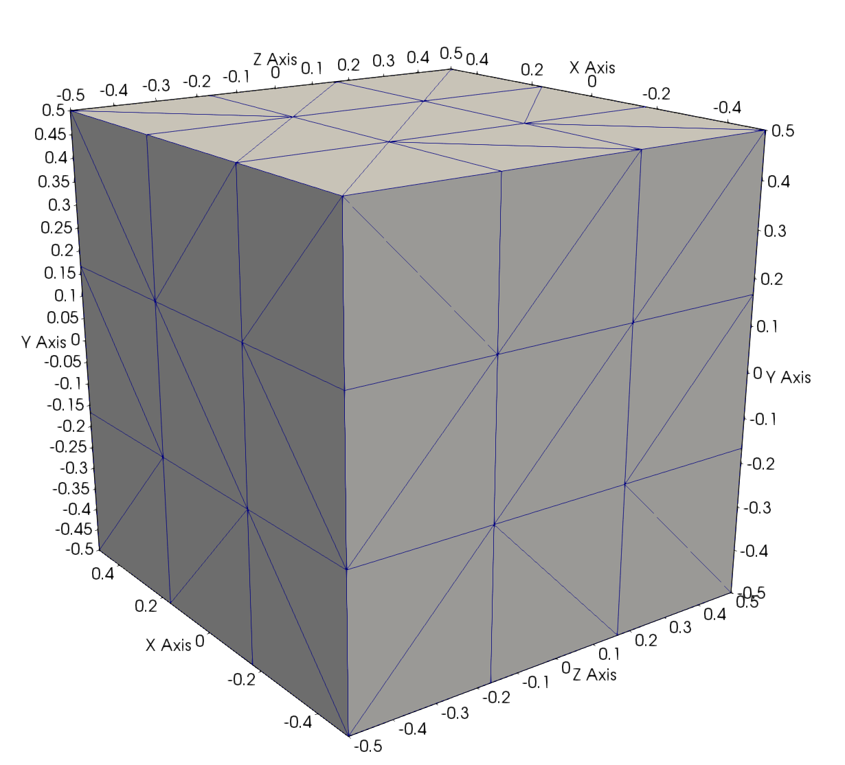
Code is executed for the mesh of a cube, see Figure 6, which has unit size for all edges and the coordinates origin is in the centre of the cube.
Code output should be similar to the following:
At the beginning the code prints the version of the MoFEM library. In the same line, versions of MOAB and PETSc libraries are printed respectively. This will enable to reproduce errors if occurred and fix bugs. Next information printed is about the name of finite elements being added, i.e. dFE, which stands for "domain finite element", and the name given to the density field, i.e. rho. For this field DOFs are added only on vertices, thus the linear approximation of density is considered. After that, the information about the number of finite elements is printed, i.e. Nb. FEs 162, the name of the problem itself, i.e. SimplePrblem, the number of DOFs on rows & columns, i.e. row dofs 64, col dofs 64, and other information related to mesh partitioning. Finally, the results are printed.
You can use your favourite editor if you have one, e.g. vim, emacs, sublime, atom.io, etc, however, if you have no preferences, we recommend VS Code. We have some tips on how you can configure it to make it work well with MoFEM, see How to configure MoFEM in Visual Studio Code?
clang-format to help us unify programming style. Most of the editors support clang-format, for example, how to do that in VS Code is described here. Keeping the same style, learning and following programming conventions is essential for the long-term development. MoFEM is an open community code, and if everyone follows the agreed style, it improves code readability, and people understand each other better.The main function is relatively short and looks the same for each program in this set of tutorials:
You can use the above snippet to start your code. The main function is responsible for kick-starting the job, and it has following stages:
Errors are caught at the end using the following code:
This part of the code is responsible for handling all errors initiated inside PETSc, MOAB, Boost, standard library, and MoFEM or developer functions. PETSc, MOAB, and MoFEM functions return error codes, to handle them properly the following macro is used:
Catching errors will make searching for runtime errors easier, and in case of the problem appearing see Guidelines for bug reporting for seeking help. CHKERR is a macro which checks error code returned by the function, and if returned code indicates an error, program stops and prints the corresponding error.
Each lesson in the tutorial series has an example class which has a very similar structure to the following:
Function Example::runProblem called by the main program has the following code:
Note that every function starts and ends with error handling
This enables stacking functions calls in case of problems. We use function stacks to see which functions, and on which lines, have been called prior to the error.
Before calculation can be performed, some bookkeeping has to be done to manage complexities related to the finite element method. MoFEM does most of this boring job "in the back-end" and only needs to be provided with initial information:
We use MoFEM::Simple interface to read command line options, load mesh file, add a field and set its order. Note that the field is added by function addDomainField and is defined by name, space, approximation base and rank. To approximate density, we choose space H1 of square-integrable functions with square-integrable derivatives and use a recipe from [1] to construct base functions, while the rank (number of coefficients) of the base is one since density is a scalar field. The order of approximation is set to one, i.e. linear base functions are used.
The common data structure is used to group the data evaluated at integration points of an element, and also to aggregate data from all elements to be used later by other parts of the code. You will find common data in all examples for the following lessons, and other parts of MoFEM implementation.
Common data structure is defined as follows:
while an instance of Example::CommonData class is created by the following method:
where memory for Example::CommonData is allocated and handled by a shared pointer. Moreover, using enable_shared_from_this and function Example::CommonData::getRhoAtIntegrationPtsPtr a shared pointer to a vector rhoAtIntegrationPtsPtr can be obtained. Finally, a PETSc vector is created and stored using MoFEM::SmartPetscObj, which is a special smart pointer for handling PETSc objects.
Smart pointers, such as boost::shared_ptr and MoFEM::SmartPetscObj, are used to maintain the life of dynamically allocated objects. You can think about smart pointers as regular C/C++ pointers, and to understand the following code you do not have to know more about them. However, more explanation is needed for the following code:
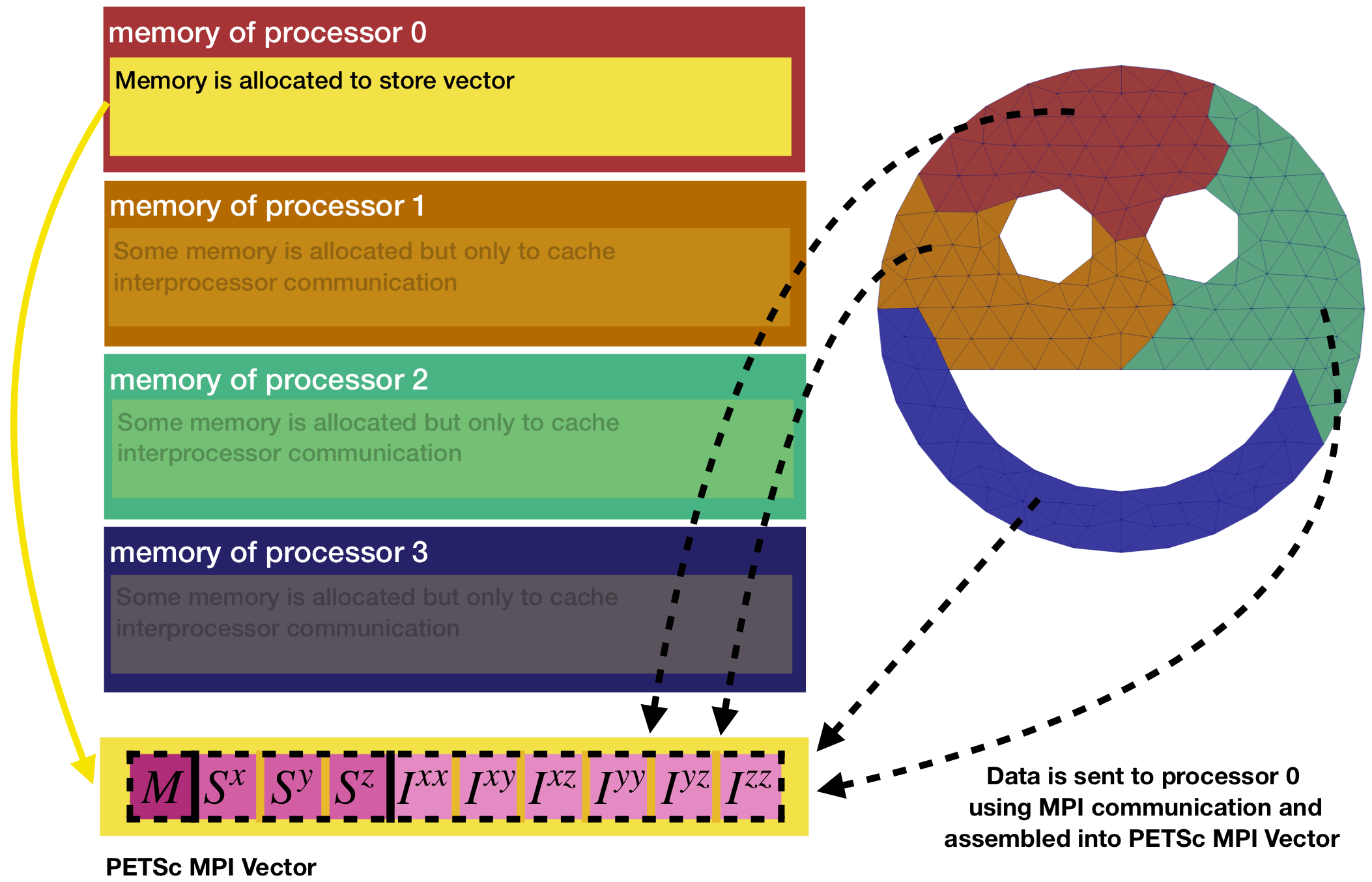
commonDataPtr->petscVec is a smart pointer to a PETSc MPI Vector, which supports access from multiple processes and is useful for parallel computing. Function MoFEM::createVectorMPI needs to be provided with a communicator, e.g. mField.get_comm(), which is a communicator of MoFEM. Communicator holds a group of processes that can communicate with each other. Next, we determine the local size of the vector which will be used to store mass, three coefficients for the first moment and six coefficients for the second moment of inertia, i.e. 10 coefficients in total in the order defined in Example::CommonData::VecElements. Note that the local size of the vector is 10 on the processor 0, and zero on other processors. It means that all data will be accumulated on processor 0 as shown in Figure 7. The global size of the vector is a sum of all local sizes, and thus is also 10.
Note that in all following lessons, including this one, we implemented code to make it work with distributed meshes.
For simplicity, density is set to unity at each node of the mesh, which represents a uniform density field. However, an arbitrary density field can be set using a small modification. Namely, function set_density in Example::setFieldValues gets coordinates as its arguments, thus you could set any density distribution you would like. Note that the MoFEM Core function MoFEM::FieldBlas::setVertexDofs is doing the hard work of setting field values to the mesh nodes. This function iterates over all nodes, gets each node's coordinates and calls the function provided by the user, i.e. set_density.
For computing moments of inertia, as well as for solving a multitude of other problems, a MoFEM developer only needs to provide the code with operators which are executed on finite element entities of the mesh. Operators can do various tasks, for example, evaluate field values at integration points, e.g. calculating \(\rho_g^h\). You will use operators as well to compute integrals when you calculate mass, the first and second moments of inertia. In other examples operators are used for calculating differential operators, e.g. gradient, divergence, etc., or assemble internal forces vector.
You would not have to write explicitly the code which integrates over finite element entities of the mesh, MoFEM will do that for you once you provide sequences (pipelines) of operators to use. There is a reason for this approach since we aim to write a finite element code which is generic and can be used in different contexts. For example, for solving a variety of problems described by Partial Differential Equations (PDEs) different solvers may be required: linear solvers, non-linear Newton-Raphson solvers, or implicit/explicit time solvers. Each solver does its own tasks iterating over finite elements. However, in MoFEM approach, a solver only has to be provided with problem specific set of operators, while the implementation of operators is independent of the type of solver.
Thus, a developer provides MoFEM with operators which are executed on each element. More precisely, these operators are executed on each sub-entity of each element, since, for example, a triangle element consists of nodes, three edges and triangle face itself. In this lesson, since density field is exclusively defined on nodes, operators are run for nodes only. However, note that this is a special case.
On each finite element, several operators can be run in a sequence. In principle, operators are used to break down a complex problem into simpler tasks. Each operator is implemented such that it iterates over integration points of an element. User-defined operators are derived from a base class UserDataOperator and have by default several basic functions which slightly vary for different element shapes. However, they always provide integration points, values of shape functions and their gradients at integrations points and finite element measures (length, area, or volume). Note that writing an operator for your problem, you do not have to make it specific for any particular element shape. In other words, the implementation of user-defined operators is independent of element shape, approximation order, and other fields used on the element, if there are any.
Shape functions on each finite element can be different, depending on approximation spaces you choose to use. Moreover, shape functions will depend on base and approximation order. Similarly, the number of DOFs and DOFs values on element entities depend on the field type. In this lesson, in function Example::setupProblem we have defined density field as follows:
where the choice of space H1 means that standard conforming elements are used, while the approximation order is set to one. Conforming elements have base functions that are continuous across element edges and faces. Mathematically speaking, function in space H1 is piecewise continuous, i.e. it is square-integrable and gradients of the function are also square-integrable. Square-integrable means that when you calculate integral of the square of the function, it gives a finite value, rather than \(\pm\infty\), i.e. the result is a real number. Approximation order 1 means that base functions are linear piecewise continuous. To build approximation base, we are using recipe AINSWORTH_LEGENDRE_BASE, which is described in details in [4]. However, since we use only the first order, shape functions are no different from those presented in Figure 4.
Our main task in this lesson is to calculate the mass, the first moment of inertia and the second moment of inertia. In order to do that, on each element we have to first calculate density at integration points, and then integrate it to obtain moments of inertia. That is depicted in Figure 8 by user data operators (UDOs) shown by four green boxes. Figure 8 also depicts the flow of data between operators through Example::CommonData structure.
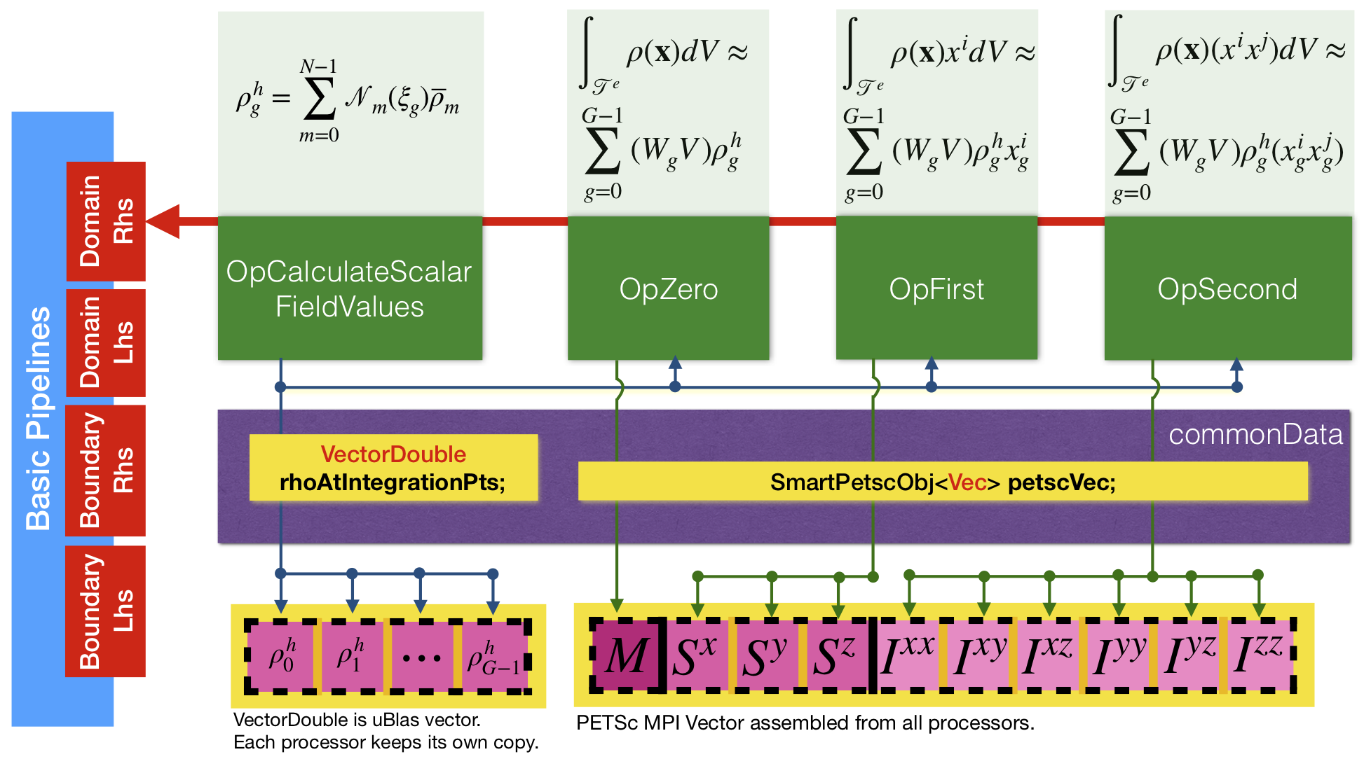
On each element, first operator MoFEM::OpCalculateScalarFieldValues is used to calculate values of density at integration points and store them in Example::CommonData::rhoAtIntegrationPts, which is a vector with a size equal to the number of integration points on the element. Then operators Example::OpZero, Example::OpFirst, and Example::OpSecond are used to evaluate moments, assembling their values to Example::CommonData::petscVec. Once all elements are iterated, vector Example::CommonData::petscVec results are printed at the end of the program.
To compute moments of inertia in MoFEM, you can use the MoFEM::PipelineManager interface, which provides pipelines where the discussed above operators can be pushed. More precisely, MoFEM::PipelineManager has several streams of pipelines to evaluate matrices and vectors for a more general class of problems, and these pipelines can be executed on domain or boundary (skin) elements. In the present tutorial we evaluate a vector by iterating domain elements, see Figure 8, red box on the left. Operators are pushed to the pipeline by executing the following code:
In the snippet above, you can see four operators pushed into the pipeline, as described in Figure 8. Operators are pushed to pipeline_mng->getOpDomainRhsPipeline, which is a pipeline to calculate vectors on domain finite elements. Note that operators are executed on each finite element in the order that they are pushed to the pipeline.
To set integration points at which base functions are evaluated, the user needs to specify integration rule, which is done by the following code:
Function integration_rule provides this rule, which is defined as the highest polynomial order under the integral for a given problem. Here the integration rule equals to the approximation order of the density field plus 2: for the second moment of inertia the function under integral is a polynomial of order \(p+2\), where p is the order of the polynomial used to approximate density, and 2 emerge from the term \(x^ix^j\). This is the highest polynomial evaluated out of three operators, therefore the integration rule set as above enables to calculate three moments of inertia exactly, and the only errors come from geometry approximation and approximation of the density by a piecewise polynomial.
Since we use a piecewise linear polynomial to approximate density, i.e. \(p=1\), the integration rule set by the code will be 3. Note that setting integration rule to a higher value would increase the number of integration points, and that will not change results. However, setting higher integration rule than is needed makes code slower since functions have to be evaluated in more points, and CPU has to do more operations.
Once the problem is set up and user operators are pushed to an appropriate pipeline, the calculation can be triggered in the function
in particular, by MoFEM::PipelineManager::loopFiniteElements. This is where all computations are happening, while the rest of the code is declaration and definition of the problem. The snippet above shows as well that vector of moments, i.e. Example::CommonData::petscVec, is zeroed before the loop over all elements is performed, and finally PETSCc functions are called to appropriately finalise assembly of an MPI Vector.
Operator Example::OpSecond is defined as follows:
Operators are derived classes, where essential part is an overloaded function Example::OpSecond::doWork, which is called by MoFEM::PipelineManager::loopFiniteElements on each finite element:
We will discuss this operator since it is the most complex one among all three operators. We will dissect this code to understand it better. We start by getting a number of integration points, which depends on the previously set integration rule. In the following lines, three tensors are declared: two rank zero (scalar) tensors are set to integration weights and density values, respectively, and a tensor of rank one (vector) is set to coordinates of integration points. Note that we use here FTensor library, providing special tools to simplify data storage and operations with tensors, you can find more details here. In particular, three tensors declared above initially point to the respective values at the first integration point, however, subsequently they will iterate through all the integration points of the element using the following code:
Next, we create an array to store local values of the second moment of inertia. The second moment of inertia is a symmetric tensor of rank two, which in three dimensions has six independent components. The array is continuous in the memory, it takes the shape of the rank two tensor when the following code is run:
With all above at hand finally the loop over all integration points is performed, and the components of the second order tensor are computed. Note that at the following line:
iteration over all 6 components of the symmetric second order tensor is performed using the special FTensor indices i and j defined before integration points loop as:
After the loop over integration points is finished, local element vector element_local_value is assembled into a global vector Example::CommonData::petscVec. Note that vector Example::CommonData::petscVec stores all moments of inertia: first index stores the zero moment, i.e. mass, next three indices store the first moment, and last six indices store the second moment. For clarity, indices are enumerated by Example::CommonData::VecElements.
The whole MoFEM code is tested every time changes are pushed into the repository. The user can also trigger the test locally using the following command:
In particular, the code in this tutorial is tested by executing
and code is validated in function Example::checkResults.
In function Example::checkResults test is run for a well-known solution for mesh in cube.h5m. Test like this verifies if mass (or volume in case of unit density), first moment and the second moment are calculated correctly. Function testing the code is as follows
You can see that at line
we check if the test option is set in the command line. Code in brackets verifies if prescribed values are equal to calculated values. For example
iterates over diagonal values of the second order tensor, and if the calculated value is not equal to expected value,program throws an error using PTESc function SETERRQ2. The test is written for a cube volume, of size one by one and coordinate system in the centre of the cube. Zero moment, i.e. volume in case of unit density, should be 1. First moments should be zero since the cube centre is placed at the origin. Diagonal values of the second-order moment should be \(1/12\), and off-diagonal terms of second-order should be zero since the sides of the cube are aligned with the axis of the coordinate system.
Writing a test for each part of the code is essential. MoFEM is a complex system with multiple contributors, and most of them focus their attention on one part of the code. Running tests like this one, contributors know that they have not broken anything. That makes code development sustainable. Also, writing tests makes code development faster and simpler, since once you have written the code, it will need refactoring and improvement. The test will reassure you that optimisations and changes do not break a working code. Moreover, once your commits are submitted to the repository, MoFEM Jenkins server will run the test independently, validating if your code is running on other systems and computers. Results of that test are available here http://cdash.eng.gla.ac.uk/cdash/index.php.
Debugging is a method used to find errors or to understand what code does. A debugger is a program for debugging, which enables the user to execute code line by line and observe, or break (stop) program at desired lines of the source code. When you work in Linux, you can use GDB to debug code. If you work on macOS, you can instead use LLDB debugger.
Code has to be compiled with debugging flags, and when you installed MoFEM using script for developer, code with debugging flags is available in $HOME/mofem_install/um/build_debug/tutorials/fun-1.
VS Code has built-in functionality to debug code, both on Linux and macOS, for details on how to use it, see https://code.visualstudio.com/docs/editor/debugging. Here is an example of the launch (in VS Code) configuration for LLDB and example from this lesson
The full source code is available here integration.cpp .
