- Note
- Prerequisites of this tutorial include MSH-1: Create a 2D mesh from Gmsh
- Note
- Intended learning outcome:
- general structure of a program developed using MoFEM
- idea of Simple Interface in MoFEM and how to use it
- solving eigen problem
- Use of form integrators
- How to push the developed UDOs to the Pipeline
Introduction
Schematic of the problem
In this tutorial, we solve a basic quantum-mechanical problem: the Schrödinger equation in a 2D infinite potential well. Below is the interactive visualization of the electron in an infinite potential well.
Electron in an Infinite Potential Well
Figure 1: Interactive simulation of the wave function and probability distribution inside the potential well.
Problem Statement
The following equation describes the dynamics of the spatial probability distribution of electrons:
\[
\begin{equation}
H(\mathbf{r},t)\psi(\mathbf{r},t)
= \mathrm{i}\hbar\frac{\partial}{\partial t}\psi(\mathbf{r},t),
\label{eq:time_dep_sch}
\end{equation}
\]
where \( \hbar \) is the reduced Planck constant. The wave function \( \psi \) describes an electron, and its squared absolute value gives the spatial probability density. The Hamiltonian operator \( H \) is defined as
\[
\begin{equation}
H(\mathbf{r},t)=-\frac{\hbar^2}{2m}\nabla^2+V(\mathbf{r},t),
\label{eq:time_H}
\end{equation}
\]
where \( m \) is the electron mass. The first term on the right-hand side of Eq. \( \eqref{eq:time_H} \) represents the kinetic energy, and the second term \( V(\mathbf{r},t) \) represents the potential energy from the electrical field. Given a steady state when \( V \) does not evolve with time, \( H \) is purely space-dependent. Consequently, the wave function \( \psi \) can be separated into a purely time-dependent part and a space-dependent part. In the time-dependent phase part, a constant \( E \) is used to describe the rate of change of the wave function, which is the system energy:
\[
\begin{equation}
\psi(\mathbf{r},t)=\psi(\mathbf{r})e^{-\mathrm{i}Et/\hbar}.
\label{eq:wave_func_sep}
\end{equation}
\]
Here \(E\) takes the same role as angular frequency in classical mechanics, as in quantum mechanics the energy of the (quasi-)particle is related to angular frequency by the constant \(\hbar\). Replacing \(H(\mathbf{r},t)\) with \(H(\mathbf{r})\) and substituting Eq. \eqref{eq:wave_func_sep} into Eq. \eqref{eq:time_dep_sch}, we get the time-independent Schrödinger equation:
\[
\begin{equation}
H(\mathbf{r})\psi(\mathbf{r})=E\psi(\mathbf{r}),
\label{eq:time_ind_sch}
\end{equation}
\]
where \( H(\mathbf{r})=-\frac{\hbar^2}{2m}\nabla^2+V(\mathbf{r}) \). Therefore, \( E \) is the eigenvalue of \( H \), and \( \psi \) is the corresponding eigenfunction. Thus, the problem of solving for the wave function reduces to solving an eigenvalue problem.
For a 2D square infinite potential well, the potential on the boundary is infinitely large for electrons to exist there (see the 1D case shown in Figure 1 where the potential is infinite at both sides of the well). Therefore, the probability density of electrons must vanish on the boundary. The strong form is
\[
\begin{align}
\label{eq:schro_strong_form_domain}
\left(-\frac{\hbar^2}{2m}\nabla^2+V(\mathbf{r})\right)\psi(\mathbf{r})
&= E\psi(\mathbf{r}), && \text{in } \Omega, \\[2mm]
\label{eq:schro_strong_form_boundary}
\psi(\mathbf{r}) &= 0, && \text{on } \Gamma.
\end{align}
\]
With the strong form given in Eq. \( \eqref{eq:schro_strong_form_domain} \) and Eq. \( \eqref{eq:schro_strong_form_boundary} \), the weak form can be derived:
find \( \psi \in \mathrm{H}^1_0(\Omega) \) such that
\[
\begin{equation}
-\frac{\hbar^2}{2m}
\int_{\Gamma}\delta\psi\nabla\psi\cdot\vec{n}\,\mathrm{d}\Gamma
+ \frac{\hbar^2}{2m}
\int_{\Omega}\nabla(\delta\psi)\nabla\psi\,\mathrm{d}\Omega
+ \int_{\Omega}\delta\psi V(\mathbf{r})\psi\,\mathrm{d}\Omega
=
E\int_{\Omega}\delta\psi\psi\,\mathrm{d}\Omega
\quad
\forall \delta\psi \in \mathrm{H}^1_0(\Omega).
\label{eq:schro_weak}
\end{equation}
\]
Here \( \mathrm{H}^1_0(\Omega) \) denotes a subspace of \( H^1(\Omega) \) consisting of functions that are set to zero on the Dirichlet boundary. Therefore, the boundary integral in Eq. \( \eqref{eq:schro_weak} \) vanishes. To compare with a case where analytical solutions are available, this tutorial assumes \( V(\mathbf{r})=0 \).
Discrete Form
To get the discrete form, we approximate the test and trial functions by the following basis functions:
\[
\begin{equation}
\delta\psi=\sum_{i=1}^{n}N_i\delta\bar{\psi}_i,
\end{equation}
\]
\[
\begin{equation}
\psi=\sum_{j=1}^{n}N_j\bar{\psi}_j.
\end{equation}
\]
Therefore, the discrete form is
\[
\begin{equation}
\sum_{j=1}^{n}
\frac{\hbar^2}{2m}
\int_{\Omega}\nabla N_i\nabla N_j\,\mathrm{d}\Omega\;\bar{\psi}_{j}
=
\sum_{j=1}^{n}
E\int_{\Omega}N_iN_j\,\mathrm{d}\Omega\;\bar{\psi}_{j},
\quad \forall i=1,2,\ldots,n.
\end{equation}
\]
By substituting
\[
\begin{equation}
H_{ij}=\frac{\hbar^2}{2m}
\int_{\Omega}\nabla N_i\nabla N_j\,\mathrm{d}\Omega,
\label{eq:H_matrix}
\end{equation}
\]
\[
\begin{equation}
M_{ij}=\int_{\Omega}N_iN_j\,\mathrm{d}\Omega,
\label{eq:M_matrix}
\end{equation}
\]
the problem reduces to the generalized eigenvalue problem
\[
\begin{equation}
[H]\bar{\psi}=E[M]\bar{\psi},
\label{eq:matrix_total}
\end{equation}
\]
where the scalar \( E \) is the eigenvalue.
Implementation
Physical Constants and Parameters
The involved physical constants and parameters are clarified below.
double hbar = 1.054571817e-34;
double m0 = 9.1093837015e-31;
double q = 1.602176634e-19;
double hbar
[Physical constants and parameters]
Boundary Condition
The infinite-potential-well boundary condition is applied by removing the DOFs associated with boundary entities using removeBlockDOFsOnEntities, which is equivalent to enforcing a zero value of the field on the boundary.
CHKERR bc_mng->removeBlockDOFsOnEntities<BcScalarMeshsetType<BLOCKSET>>(
true);
}
#define MoFEMFunctionBegin
First executable line of each MoFEM function, used for error handling. Final line of MoFEM functions ...
#define MoFEMFunctionReturn(a)
Last executable line of each PETSc function used for error handling. Replaces return()
#define CHKERR
Inline error check.
MoFEMErrorCode boundaryCondition()
[Set up problem]
MoFEM::Interface & mField
Reference to MoFEM interface.
const std::string getProblemName() const
Get the Problem Name.
MoFEMErrorCode getInterface(IFACE *&iface) const
Get interface reference to pointer of interface.
Assembling the Matrices
The \([H]\) and \([M]\) matrices are assembled by OpDomainGradGrad and OpDomainMass respectively according to Eq. \eqref{eq:H_matrix} and Eq. \eqref{eq:M_matrix}. Here pipeline_mng->getDomainLhsFE()->B = H and pipeline_mng->getDomainLhsFE()->A = M are used to store the assembled matrices into \([H]\) and \([M]\), respectively. As SLEPC's EPS solver is not deeply integrated with PETSc as KSP solvers, the two matrices need to be explicitly passed to EPS solver later.
PETSC_NULLPTR);
};
};
return 1.0;
};
auto calculate_Hamiltonian = [&]() {
pipeline_mng->getDomainLhsFE().reset();
CHKERR AddHOOps<SPACE_DIM, SPACE_DIM, SPACE_DIM>::add(
pipeline_mng->getOpDomainLhsPipeline(), {H1});
pipeline_mng->getOpDomainLhsPipeline().push_back(
pipeline_mng->getOpDomainLhsPipeline().push_back(
};
pipeline_mng->getDomainLhsFE()->B =
H;
CHKERR pipeline_mng->loopFiniteElements();
CHKERR MatAssemblyBegin(
H, MAT_FINAL_ASSEMBLY);
CHKERR MatAssemblyEnd(
H, MAT_FINAL_ASSEMBLY);
};
auto calculate_mass_matrix = [&]() {
pipeline_mng->getDomainLhsFE().reset();
CHKERR AddHOOps<SPACE_DIM, SPACE_DIM, SPACE_DIM>::add(
pipeline_mng->getOpDomainLhsPipeline(), {H1});
pipeline_mng->getOpDomainLhsPipeline().push_back(
};
pipeline_mng->getDomainLhsFE()->B =
M;
CHKERR pipeline_mng->loopFiniteElements();
CHKERR MatAssemblyBegin(
M, MAT_FINAL_ASSEMBLY);
CHKERR MatAssemblyEnd(
M, MAT_FINAL_ASSEMBLY);
};
CHKERR calculate_Hamiltonian();
CHKERR calculate_mass_matrix();
}
FormsIntegrators< DomainEleOp >::Assembly< PETSC >::BiLinearForm< GAUSS >::OpMass< 1, FIELD_DIM > OpDomainMass
PetscErrorCode DMCreateMatrix_MoFEM(DM dm, Mat *M)
FormsIntegrators< DomainEleOp >::Assembly< PETSC >::BiLinearForm< GAUSS >::OpGradGrad< 1, 1, SPACE_DIM > OpDomainGradGrad
PetscErrorCode PetscOptionsGetScalar(PetscOptions *, const char pre[], const char name[], PetscScalar *dval, PetscBool *set)
SmartPetscObj< Mat > matDuplicate(Mat mat, MatDuplicateOption op)
static constexpr int approx_order
MoFEMErrorCode assembleSystem()
[Push operators to pipeline]
MoFEMErrorCode getDM(DM *dm)
Get DM.
Solving the Eigenvalue Problem
An EPS solver is created by EPSCreate(comm, &eps), with \(H\) as the left-hand-side stiffness matrix and \([M]\) as the right-hand-side mass matrix to solve the problem. The option EPS_GHEP specifies we are solving a generalized Hermitian eigenvalue problem. By 'generalized' it means an additional mass matrix on the right-hand side, and by 'Hermitian' it means the left-hand-side matrix \([H]\) is equal to its complex conjugate transpose. EPS_SMALLEST_MAGNITUDE instructs the solver to compute the eigenvalues starting from the smallest. Parameter settings for the solver are printed out for reference during execution. From its we can see the number of iterations taken by the solver to converge, and nev indicates the number of eigenvalues that will be computed within the specified tolerance tol. type indicates the method being used in the solver, which in this tutorial is Krylov-Schur method.
auto create_eps = [](MPI_Comm
comm) {
return SmartPetscObj<EPS>(
eps);
};
auto setup_eps = [&]() {
CHKERR EPSSetWhichEigenpairs(
eps, EPS_SMALLEST_MAGNITUDE);
PetscInt nev = 20;
EPSSetDimensions(
eps, nev, PETSC_DEFAULT, PETSC_DEFAULT);
};
auto print_info = [&]() {
ST st;
PetscInt nev, maxit, its;
" Number of iterations of the method: %d", its);
CHKERR EPSGetDimensions(
eps, &nev, NULL, NULL);
MOFEM_LOG_C(
"EXAMPLE", Sev::inform,
" Number of requested eigenvalues: %d",
nev);
" Stopping condition: tol=%.4g, maxit=%d", (
double)
tol, maxit);
};
}
#define MOFEM_LOG_C(channel, severity, format,...)
MoFEMErrorCode solveSystem()
[Solve]
virtual MPI_Comm & get_comm() const =0
Postprocessing
The eigenpairs are retrieved by EPSGetEigenpair, where nn indicates the index of the eigenpair, eigr/eigi indicates the real/imaginary part of the eigenvalue, and D receives the real part of the corresponding eigenvector. Since in this tutorial the wave functions are composed of real-valued sine functions, only the real parts of the eigenvectors are stored. Besides, as \([H]\) is Hermitian, the eigenvalues are real as well, so only eigr is stored. The wave function PHI is obtained from D, and the square of the wave function is calculated by OpSquare operator.
pipeline_mng->getDomainLhsFE().reset();
auto post_proc_fe = boost::make_shared<PostProcEle>(
mField);
auto phi_ptr = boost::make_shared<VectorDouble>();
auto square_ptr = boost::make_shared<VectorDouble>();
post_proc_fe->getOpPtrVector().push_back(
new OpCalculateScalarFieldValues("PHI", phi_ptr));
post_proc_fe->getOpPtrVector().push_back(new OpSquare(
square_ptr,
phi_ptr));
using OpPPMap = OpPostProcMapInMoab<SPACE_DIM, SPACE_DIM>;
post_proc_fe->getOpPtrVector().push_back(
new OpPPMap(post_proc_fe->getPostProcMesh(),
post_proc_fe->getMapGaussPts(),
OpPPMap::DataMapVec{{"PHI", phi_ptr}, {"SQUARE", square_ptr}},
);
pipeline_mng->getDomainRhsFE() = post_proc_fe;
PetscInt nev, nconv, n_output = 0;
CHKERR EPSGetDimensions(
eps, &nev, PETSC_NULLPTR, PETSC_NULLPTR);
n_output = std::min(nconv, nev);
if (nconv < nev) {
" Only %" PetscInt_FMT " of %" PetscInt_FMT
" requested eigenpairs converged",
nconv, nev);
}
PetscScalar eigr, eigi;
for (PetscInt nn = 0; nn < n_output; nn++) {
CHKERR EPSGetEigenpair(
eps, nn, &eigr, &eigi,
D, PETSC_NULLPTR);
CHKERR VecGhostUpdateBegin(
D, INSERT_VALUES, SCATTER_FORWARD);
CHKERR VecGhostUpdateEnd(
D, INSERT_VALUES, SCATTER_FORWARD);
" Eigenpair = %" PetscInt_FMT " Eigen Energy = %.8g eV", nn,
CHKERR pipeline_mng->loopFiniteElements();
post_proc_fe->writeFile("out_schrod_" +
boost::lexical_cast<std::string>(nn) + ".h5m");
}
}
void simple(double P1[], double P2[], double P3[], double c[], const int N)
PetscErrorCode DMoFEMMeshToLocalVector(DM dm, Vec l, InsertMode mode, ScatterMode scatter_mode, RowColData rc=RowColData::COL)
set local (or ghosted) vector values on mesh for partition only
auto createDMVector(DM dm, RowColData rc=RowColData::COL)
Get smart vector from DM.
OpPostProcMapInMoab< SPACE_DIM, SPACE_DIM > OpPPMap
MoFEMErrorCode outputResults()
[Solve]
std::map< std::string, boost::shared_ptr< MatrixDouble > > DataMapMat
Definition of Operator
In this operator we calculate the square of the wave function per Gauss point, which is the probability density of electrons.
struct OpSquare : public ForcesAndSourcesCore::UserDataOperator {
OpSquare(boost::shared_ptr<VectorDouble> squareField,
boost::shared_ptr<VectorDouble> field)
squareField(squareField), field(field) {}
MoFEMErrorCode doWork(
int side, EntityType
type,
DataForcesAndSourcesCore::EntData &data) {
const size_t nb_gauss_pts = getGaussPts().size2();
squareField->resize(nb_gauss_pts, 0);
auto t_squareField = getFTensor0FromVec(*squareField);
auto t_field = getFTensor0FromVec(*field);
for (int gg = 0; gg != nb_gauss_pts; gg++) {
t_squareField = t_field * t_field;
++t_field;
++t_squareField;
}
}
private:
boost::shared_ptr<VectorDouble> squareField;
boost::shared_ptr<VectorDouble> field;
};
ForcesAndSourcesCore::UserDataOperator UserDataOperator
Results
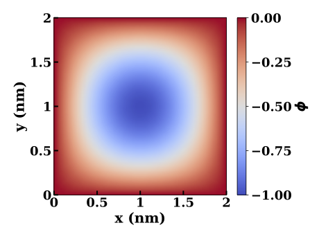
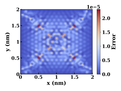
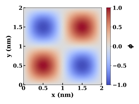
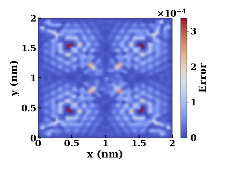
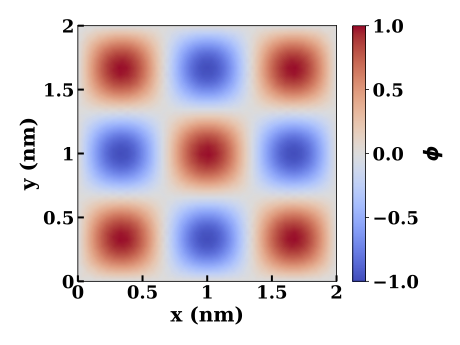
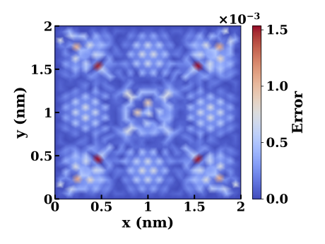
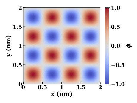
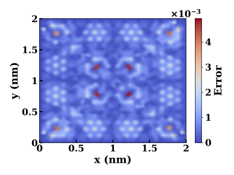
In quantum mechanics, the analytical solutions for electrons in a 2D square infinite potential well of length of \(L\) are: \begin{equation} \label{eq:E_theo} E_{n_x,n_y}=\frac{\hbar^2 \pi^2}{2mL^2}(n_x^2+n_y^2),\quad n_x,n_y=1,2,3,... \end{equation} \begin{equation} \label{eq:phi_theo} \psi_{n_x,n_y}(x,y)=\frac{2}{L}\text{sin}\left(\frac{n_x\pi x}{L}\right)\text{sin}\left(\frac{n_y\pi y}{L}\right),\quad n_x,n_y=1,2,3,... \end{equation} With \(L=2\) nm, \(E\) takes the form \(0.09401*(n_x^2+n_y^2)\) eV. Each \((n_x,n_y)\) quantum number pair corresponds to a unique quantum state. As indicated by Eq. \eqref{eq:E_theo}, degenerate states exist, which means a single energy level may accommodate electrons in multiple quantum states. In Table 1, the numerical eigenenergies computed by MoFEM are compared with the analytical solutions in Eq. \eqref{eq:E_theo}. The degeneracy describes the number of linearly independent eigenfunctions corresponding to the same eigenvalue, namely the number of quantum states with the same energy, and non-degenerate states have a degeneracy of 1. Similarly, Figure 2 shows the space-resolved wave functions from MoFEM and compares them with the theoretical expressions given in Eq. \eqref{eq:phi_theo}. The numerical results for both eigenenergies and eigenfunctions are consistent with what is predicted by quantum mechanical theory. The reason why only the wave functions corresponding to non-degenerate energy levels are shown in Figure 2 is that exact closed-form analytical expressions are available only in these cases. In degenerate cases, the eigenvectors merely span a subspace, and any orthonormal basis of that subspace is mathematically valid.
Table 1: the 20 smallest eigenenergies
| Quantum State (n_x,n_y) | Degeneracy | Analytical results (eV) | MoFEM (eV) |
| (1,1) | 1 | 0.18802 | 0.18802 |
| (1,2),(2,1) | 2 | 0.47004 | 0.47005, 0.47005 |
| (2,2) | 1 | 0.75206 | 0.75211 |
| (1,3),(3,1) | 2 | 0.94008 | 0.94019, 0.94020 |
| (2,3),(3,2) | 2 | 1.22210 | 1.22236, 1.22237 |
| (1,4),(4,1) | 2 | 1.59813 | 1.59871, 1.59872 |
| (3,3) | 1 | 1.69214 | 1.69278 |
| (2,4),(4,2) | 2 | 1.88015 | 1.88103, 1.88112 |
| (3,4),(4,3) | 2 | 2.35019 | 2.35195, 2.35120 |
| (1,5),(5,1) | 2 | 2.44420 | 2.44621, 2.44625 |
| (2,5),(5,2) | 2 | 2.72622 | 2.72892, 2.72898 |
| (4,4) | 1 | 3.00824 | 3.01188 |
(a) Wave function for the first eigenmode |
(b) Error of the first eigenmode |
(d) Wave function for the fourth eigenmode |
(e) Error of the fourth eigenmode |
(d) Wave function for the eleventh eigenmode |
(e) Error of the eleventh eigenmode |
(d) Wave function for the twentieth eigenmode |
(e) Error of the twentieth eigenmode |
Figure 2: The wave functions and their corresponding errors.
Source code
Main Program (cpp)
#ifndef EXECUTABLE_DIMENSION
#define EXECUTABLE_DIMENSION 2
#endif
#undef EPS
#include <slepceps.h>
};
};
double hbar = 1.054571817e-34;
double m0 = 9.1093837015e-31;
double q = 1.602176634e-19;
static char help[] =
"...\n\n";
private:
};
}
}
}
true);
}
PETSC_NULLPTR);
};
};
return 1.0;
};
auto calculate_Hamiltonian = [&]() {
pipeline_mng->getDomainLhsFE().reset();
pipeline_mng->getOpDomainLhsPipeline(), {H1});
pipeline_mng->getOpDomainLhsPipeline().push_back(
pipeline_mng->getOpDomainLhsPipeline().push_back(
};
pipeline_mng->getDomainLhsFE()->B =
H;
CHKERR pipeline_mng->loopFiniteElements();
CHKERR MatAssemblyBegin(
H, MAT_FINAL_ASSEMBLY);
CHKERR MatAssemblyEnd(
H, MAT_FINAL_ASSEMBLY);
};
auto calculate_mass_matrix = [&]() {
pipeline_mng->getDomainLhsFE().reset();
pipeline_mng->getOpDomainLhsPipeline(), {H1});
pipeline_mng->getOpDomainLhsPipeline().push_back(
};
pipeline_mng->getDomainLhsFE()->B =
M;
CHKERR pipeline_mng->loopFiniteElements();
CHKERR MatAssemblyBegin(
M, MAT_FINAL_ASSEMBLY);
CHKERR MatAssemblyEnd(
M, MAT_FINAL_ASSEMBLY);
};
CHKERR calculate_Hamiltonian();
CHKERR calculate_mass_matrix();
}
auto create_eps = [](MPI_Comm
comm) {
};
auto setup_eps = [&]() {
CHKERR EPSSetWhichEigenpairs(
eps, EPS_SMALLEST_MAGNITUDE);
PetscInt nev = 20;
EPSSetDimensions(
eps, nev, PETSC_DEFAULT, PETSC_DEFAULT);
};
auto print_info = [&]() {
ST st;
PetscInt nev, maxit, its;
" Number of iterations of the method: %d", its);
CHKERR EPSGetDimensions(
eps, &nev, NULL, NULL);
MOFEM_LOG_C(
"EXAMPLE", Sev::inform,
" Number of requested eigenvalues: %d",
nev);
" Stopping condition: tol=%.4g, maxit=%d", (
double)
tol, maxit);
};
}
auto post_proc_fe = boost::make_shared<PostProcEle>(
mField);
auto phi_ptr = boost::make_shared<VectorDouble>();
auto square_ptr = boost::make_shared<VectorDouble>();
post_proc_fe->getOpPtrVector().push_back(
post_proc_fe->getOpPtrVector().push_back(
new OpSquare(
square_ptr,
phi_ptr));
post_proc_fe->getOpPtrVector().push_back(
new OpPPMap(post_proc_fe->getPostProcMesh(),
post_proc_fe->getMapGaussPts(),
);
pipeline_mng->getDomainRhsFE() = post_proc_fe;
PetscInt nev, nconv, n_output = 0;
CHKERR EPSGetDimensions(
eps, &nev, PETSC_NULLPTR, PETSC_NULLPTR);
n_output = std::min(nconv, nev);
if (nconv < nev) {
" Only %" PetscInt_FMT " of %" PetscInt_FMT
" requested eigenpairs converged",
nconv, nev);
}
PetscScalar eigr, eigi;
for (PetscInt nn = 0; nn < n_output; nn++) {
CHKERR EPSGetEigenpair(
eps, nn, &eigr, &eigi,
D, PETSC_NULLPTR);
CHKERR VecGhostUpdateBegin(
D, INSERT_VALUES, SCATTER_FORWARD);
CHKERR VecGhostUpdateEnd(
D, INSERT_VALUES, SCATTER_FORWARD);
" Eigenpair = %" PetscInt_FMT " Eigen Energy = %.8g eV", nn,
CHKERR pipeline_mng->loopFiniteElements();
post_proc_fe->writeFile("out_schrod_" +
boost::lexical_cast<std::string>(nn) + ".h5m");
}
}
PetscBool test_flg = PETSC_FALSE;
PETSC_NULLPTR);
if (test_flg) {
PetscInt nconv;
if (nconv < 1) {
"No eigenpairs converged");
}
PetscScalar eigr, eigi;
CHKERR EPSGetEigenpair(
eps, 0, &eigr, &eigi, PETSC_NULLPTR, PETSC_NULLPTR);
constexpr double regression_value =
0.188;
if (fabs(eigr /
q - regression_value) > 1e-3) {
PetscPrintf(PETSC_COMM_WORLD,
"Calculated ground energy: %.4g, expected %.4g\n",
(
double)eigr /
q, regression_value);
"Regression test faileed; wrong eigen value. Try higher order or "
"finer mesh.");
}
}
}
int main(
int argc,
char *argv[]) {
const char param_file[] = "param_file.petsc";
SlepcInitialize(&argc, &argv, param_file,
help);
auto core_log = logging::core::get();
core_log->add_sink(
LogManager::createSink(LogManager::getStrmWorld(), "EXAMPLE"));
LogManager::setLog("EXAMPLE");
try {
DMType dm_name = "DMMOFEM";
moab::Core mb_instance;
moab::Interface &moab = mb_instance;
}
SlepcFinalize();
}
ElementsAndOps< SPACE_DIM >::DomainEle DomainEle
#define CATCH_ERRORS
Catch errors.
@ AINSWORTH_BERNSTEIN_BEZIER_BASE
@ MOFEM_ATOM_TEST_INVALID
PetscErrorCode DMRegister_MoFEM(const char sname[])
Register MoFEM problem.
#define MOFEM_LOG(channel, severity)
Log.
#define MOFEM_LOG_TAG(channel, tag)
Tag channel.
MoFEMErrorCode removeBlockDOFsOnEntities(const std::string problem_name, const std::string block_name, const std::string field_name, int lo, int hi, bool get_low_dim_ents=true, bool is_distributed_mesh=true)
Remove DOFs from problem based on block entities.
PetscErrorCode MoFEMErrorCode
MoFEM/PETSc error code.
implementation of Data Operators for Forces and Sources
PetscErrorCode PetscOptionsGetInt(PetscOptions *, const char pre[], const char name[], PetscInt *ivalue, PetscBool *set)
PetscErrorCode PetscOptionsGetBool(PetscOptions *, const char pre[], const char name[], PetscBool *bval, PetscBool *set)
#define EXECUTABLE_DIMENSION
Calculate the square of wave function.
MoFEMErrorCode readMesh()
[Run problem]
MoFEMErrorCode checkResults()
[Postprocess results]
MoFEMErrorCode runProblem()
[Run problem]
MoFEMErrorCode setupProblem()
[Run problem]
Add operators pushing bases from local to physical configuration.
Boundary condition manager for finite element problem setup.
Template specialization for scalar field boundary conditions.
static MoFEMErrorCode Initialize(int *argc, char ***args, const char file[], const char help[])
Initializes the MoFEM database PETSc, MOAB and MPI.
static MoFEMErrorCode Finalize()
Checks for options to be called at the conclusion of the program.
Deprecated interface functions.
Specialization for double precision scalar field values calculation.
Post post-proc data at points from hash maps.
std::map< std::string, ScalarDataPtr > DataMapVec
PipelineManager interface.
boost::shared_ptr< FEMethod > & getDomainLhsFE()
Get domain left-hand side finite element.
Simple interface for fast problem set-up.
MoFEMErrorCode addDomainField(const std::string name, const FieldSpace space, const FieldApproximationBase base, const FieldCoefficientsNumber nb_of_coefficients, const TagType tag_type=MB_TAG_SPARSE, const enum MoFEMTypes bh=MF_ZERO, int verb=-1)
Add field on domain.
MoFEMErrorCode loadFile(const std::string options, const std::string mesh_file_name, LoadFileFunc loadFunc=defaultLoadFileFunc)
Load mesh file.
MoFEMErrorCode getOptions()
get options
MoFEMErrorCode setFieldOrder(const std::string field_name, const int order, const Range *ents=NULL)
Set field order.
MoFEMErrorCode setUp(const PetscBool is_partitioned=PETSC_TRUE)
Setup problem.
intrusive_ptr for managing petsc objects
Volume finite element base.
[Calculate square of wave function]
Operator (hpp)
boost::shared_ptr<VectorDouble>
field)
DataForcesAndSourcesCore::EntData &data) {
const size_t nb_gauss_pts = getGaussPts().size2();
auto t_field = getFTensor0FromVec(*
field);
for (int gg = 0; gg != nb_gauss_pts; gg++) {
t_squareField = t_field * t_field;
++t_field;
++t_squareField;
}
}
private:
boost::shared_ptr<VectorDouble>
field;
};
}
structure to get information from mofem into EntitiesFieldData
boost::shared_ptr< VectorDouble > field
boost::shared_ptr< VectorDouble > squareField
MoFEMErrorCode doWork(int side, EntityType type, DataForcesAndSourcesCore::EntData &data)