 |
v0.14.0 |
|
v0.14.0 |
In this tutorial, we show how to solve a strongly nonlinear time dependent equation using mix-finite-elements. We focus on construction of finite elements, finite element user data operators (UDO), setting up discrete manager (DM) and time solver (TS). Issues related to the nonlinear solver and line searchers are briefly discussed. We also show how to use automatic differentiation (ADOL-C) to calculate derivatives of a constitutive model.
Problem solved here is similar to the solution of nonlinear Poisson's equation described in COR-5: A nonlinear Poisson equation and is a generalization of the problem described in COR-0: Mixed formulation and integration on skeleton (h-adaptivity). You might look to those tutorials if some implementation aspects of presented methodology are unclear. Also, you are encouraged to post questions on our Q&A forum.
Presented methodology is applied to the problem of unsaturated water transport. We have no intention to give a detailed description of transport in unsaturated materials, here we only focus on problem discretization, equations linearization and implementation of finite element. Also, we do not show here how to do hp-adaptivity, this is part of other tutorials. This problem can be solved with block solver, improving its efficiency and robustness, see example COR-4: Using fieldsplit solver and DM sub problem.. If you like to extend this work, adding block solver or hp-adaptivity, we offer our guidance and help.
The application for unsaturated flow is implemented in unsaturated_transport.cpp, material models are implemented in MaterialUnsaturatedFlow.hpp, problem definition and implementation are implemented in UnsaturatedFlow.hpp.
The tutorial is organized as follows. First, we explain how to run the application. Next, we show how the material model is implemented, after that we explain the mathematical and numerical models. Finally, we explain implementation details.
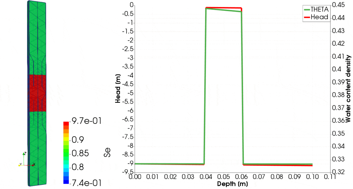
You can imagine that we do an experiment, such that we have wet silt and dry clay, we make three layers, with silt in the middle, and clay on the top and below. Such column of soil we put in the box, for example, made from plexiglass. Thus all sides are impermeable. We will observe water content and capillary pressure for two days, that is long enough to approach equilibrium.
First, we create a mesh which can be made in Salome, gMesh, Tetgen, or any other code. MoFEM uses MOAB for mesh database which can read various mesh file formats. Here we using Cubit to make the mesh, the journal file for this problem is as follows
reset
# create body volume
brick x 0.01 y 0.002 z 0.1
move Volume all x 0 y 0 z -0.05 include_merged
brick x 0.1 y 0.06 z 0.02
move Volume 2  location volume 1  include_merged
chop volume 1 with volume 2
imprint volume all
merge volume all
# make block for clay
block 1 volume 4 5
block 1 name 'SOIL_CLAY1'
# make block for silt
block 2 volume 3
block 2 name 'SOIL_SILT2'
# make mesh
volume all size auto factor 10
volume all scheme Tetmesh
mesh volume all
# refine mesh at interfaces between clay & silt
refine surface 13 14 size 0.0025 bias 1.5 depth 1 smooth
Note that we do not set any boundary conditions here, in that case, it is assumed that fluxes on the boundary are zero, that is the boundary is impermeable.
Next, we need to make a configuration file, where all problem specific parameters are set.
[mat_block_1]
# VanGenuchten
# SimpleDarcy
material_name=VanGenuchten
# Default material for VanGenuchten is Clay (no need to set parameters if clay is used)
# Assumed units are in meters and days.

# Model parameters controlling convergence
sCale=1e6       # Scale mass conservation equation
ePsilon1=1e-5   # Minimal capacity when removing spurious oscillations in time

Ah=-9 # head suction at z = 0
AhZ=1 #�gradient of initial head suction
AhZZ=0 # initial head suction is calculated from equation h = Ah + AhZZ*z + AhZZ*zz

[mat_block_2]
material_name=VanGenuchten
# Material parameters for Silt from Vogel., van Genuchten Cislerova 2001
sCale=1e6
ePsilon1=1e-5
Ah=-0.09
AhZ=1
thetaS=0.46
thetaM=0.46
thetaR=0.034
alpha=1.6
n=1.37
Ks=0.006
hS=0
The material parameters are taken from [73], the initial parameters for clay (mat_block_1) and silt (mat_block_2) are set with the \(A_h\) and \(A_h^z\), such that initial capillary pressure head is given by \( h = A_h+A_h^z z \) where
\[ \left\{ \begin{array}{ll} h(z,t=0) = -9+z&\textrm{for clay}\\ h(z,t=0) = -0.09+z&\textrm{for silt} \end{array} \right. \]
The analysis is run using script run_uf.sh
Editing that file you can set range of parameters, control time solver, tolerances, stop criteria, line-searcher. For details look to PETSc manual link.
Note that here the solved problem is strongly nonlinear, and we use secant line-search in the L2 norm (see link). For stability of the result at each Newton iteration, we execute three sub-iterations with line searcher. Also, you have the option of controlling the time step adaptively and linear solver pre-conditioner. All command line options, both PETSc and MoFEM are printed if you add switch -help when you run MoFEM application.
MoFEM specific options are
Finally, we can run the simulation by executing above the script
where
For the problem setup like above, results are shown in Figure 1, where the evolution of various parameters over time until equilibrium is reached is shown. You can note that initially, clay is relatively dry, whereas silt is wet. Over time, the clay sucks the water from the silt. On the left-hand side, we observe the distribution of saturation. Initially, high gradients of pressure head are created on the interface between the two materials. Those are captured very well, despite the coarse mesh, showing capabilities of the presented problem formulation. For creation of this figure we used the 2nd order of polynomial to approximate the pressure head and the 3rd order polynomial to approximate the fluxes.
In the second example, we show how to run downward infiltration problem with three layers, i.e. clay, silt and clay.
In the case above, we apply zero pressure head and the rest of the boundary is impermeable. See the following journal script to generate such a mesh
reset
# create body volume
brick x 0.01 y 0.002 z 0.1
move Volume all x 0 y 0 z -0.05 include_merged
brick x 0.1 y 0.06 z 0.02
move Volume 2  location volume 1  include_merged
chop volume 1 with volume 2
imprint volume all
merge volume all
# make block for clay
block 1 volume 4 5
block 1 name 'SOIL_CLAY1'
# make block for silt
block 2 volume 3
block 2 name 'SOIL_SILT2'
block 3 surface 1
block 3 name 'HEAD1'
block 3 attribute count 1
block 3 attribute index 1 0
# make mesh
volume all size auto factor 10
volume all scheme Tetmesh
mesh volume all
# refine mesh at interfaces between clay & silt
refine surface 1 13 14 size 0.0025 bias 1.5 depth 1 smooth
Here we add the third block name HEAD1, where a boundary condition is applied. Similarly, non-zero fluxes can be applied by making a block with some surface elements and called it for example "FLUX1".
The material parameters are similar to the ones given in the previous problem
[mat_block_1]
# VanGenuchten
# SimpleDarcy
material_name=VanGenuchten
# Default material for VanGenuchten is Clay (no need to set parameters if clay is used)
# Assumed units are in meters and days.

# Model parameters controlling convergence
sCale=1e6       # Scale mass conservation equation
ePsilon1=1e-5   # Minimal capacity when removing spurious oscillations in time

Ah=-9 # head suction at z = 0
AhZ=1 #�gradient of initial head suction
AhZZ=0 # initial head suction is calculated from equation h = Ah + AhZZ*z + AhZZ*zz

[mat_block_2]
material_name=VanGenuchten
# Material parameters for Silt from Vogel., van Genuchten Cislerova 2001
sCale=1e6
ePsilon1=1e-5
Ah=-9
AhZ=1
thetaS=0.46
thetaM=0.46
thetaR=0.034
alpha=1.6
n=1.37
Ks=0.006
hS=0

# You can change boundary conditions here
#[head_block_3]
#head = 0
Note that for this example we set initial pressure head distribution such that clay and silt are in equilibrium.
\[ \left\{ \begin{array}{ll} h(z,t=0) = -9+z&\textrm{for clay}\\ h(z,t=0) = -9+z&\textrm{for silt} \end{array} \right. \]
Moreover at the end we show how to modify boundary condition. As an excrete one can change value of head on the top of the sample.
We run script as before
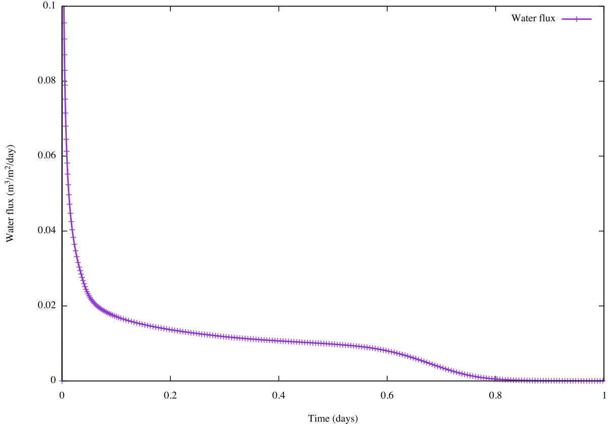
For this example, we observe an influx of water into the column of the solid, we can plot how it is changing over time. At every time step, the solver monitor prints on the screen following lines
63 TS dt 0.00242774 time 0.0710581
Flux at time 0.07106 3.859e-07
    0 SNES Function norm 4.123926528377e-02
    1 SNES Function norm 6.552371691866e-02
    2 SNES Function norm 7.740255184123e-02
    3 SNES Function norm 7.999178179888e-02
    4 SNES Function norm 7.881110800442e-02
    5 SNES Function norm 7.582982118207e-02
    6 SNES Function norm 7.173427725809e-02
    7 SNES Function norm 6.666200930695e-02
    8 SNES Function norm 6.040633270649e-02
    9 SNES Function norm 5.232159632926e-02
   10 SNES Function norm 4.057267597689e-02
   11 SNES Function norm 1.625005251310e-02
   12 SNES Function norm 4.316837250846e-05
   13 SNES Function norm 8.980432593466e-07
  Nonlinear solve converged due to CONVERGED_FNORM_RELATIVE iterations 13
      TSAdapt 'basic': step  63 accepted t=0.0710581  + 2.428e-03 wlte=0.546 family='beuler' scheme=0:'' dt=2.627e-03
64 TS dt 0.00262737 time 0.0734859
Flux at time 0.07349 3.812e-07
    0 SNES Function norm 4.023589003253e-02
    1 SNES Function norm 6.962486297267e-02
    2 SNES Function norm 8.329691099303e-02
    3 SNES Function norm 8.641640743250e-02
    4 SNES Function norm 8.532070311444e-02
    5 SNES Function norm 8.223165652333e-02
    6 SNES Function norm 7.792739113001e-02
    7 SNES Function norm 7.257891287567e-02
    8 SNES Function norm 6.598809018682e-02
    9 SNES Function norm 5.751011198160e-02
   10 SNES Function norm 4.535116560548e-02
   11 SNES Function norm 2.147388609216e-02
   12 SNES Function norm 1.073710142541e-05
   13 SNES Function norm 4.011739514453e-11
  Nonlinear solve converged due to CONVERGED_FNORM_ABS iterations 13
      TSAdapt 'basic': step  64 accepted t=0.0734859  + 2.627e-03 wlte=0.588 family='beuler' scheme=0:'' dt=2.742e-03
where for step 63 and 64, total flux is printed in \(m^3/day\),
Flux at time 0.07106 3.859e-07
Flux at time 0.07349 3.812e-07
We can extract that information using awk/grep as follows
This shell command line takes all lines which have the phrase "Flux at", takes the fourth and the fifth columns from those lines, whereas fifth column is divided by area of the surface where the head is applied. Finally, results are stored in file gp. You can plot results in MS Excel or any other software, we choose to use gnuplot. As a result, we get Figure 2 below.
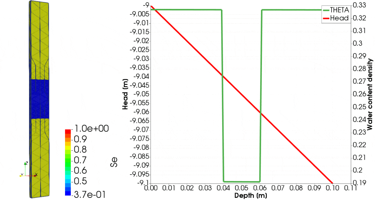
In Figure 3 below, we can observe how the wetting front is moving downwards. Note how the gradient of head differs between clay and silt, and how it moves through the interface between materials.
We consider porous material partially filled with water. In this tutorial, we are going to simulate water transport in such a system. The primary behaviour of the system depends on the material structure, capillary forces and the wetting angle, taken into account by experimentally estimated material parameters. Darcy's law gives the relation between flux and suction head (capillary pressure). Constitutive equations describe the relationship between hydraulic conductivity and water content. It is assumed that the state of the material is a function of water content, and using water retention curve one can map the between capillary head and the water content, i.e. \(\theta=\theta(h)\). The process of the water flow has to obey the conservation of mass, and consequently, the process of unsaturated transport is described by the parabolic differential equation.
The Richards equation describes the problem of unsaturated flow
\[ \frac{\partial \theta}{\partial t}- \nabla \cdot \left[ \left( K(\theta) \nabla ( h - z) \right) \right] = 0 \]
where \(z\) is depth and \(K=K(\theta)\) is hydraulic conductivity. \(\nabla\) and \(\nabla \cdot\) are differential operators for gradient and divergence respectively. The above equation can alternatively be expressed by the system of first order partial differential equations
\[ \left\{ \begin{array}{l} \frac{1}{K(\theta)}\boldsymbol\sigma + \nabla (h -z) = 0 \\ c(\theta)\frac{\partial h}{\partial t} - \nabla \cdot \boldsymbol\sigma = 0 \end{array} \right. \]
where \(\boldsymbol\sigma\) is flux. The first equation expresses the constitutive relation while the second is the conservation law. The second equation is also called the continuity equation, and it does not allow for creation or annihilation of mass. The capacity term \(c\) in the second equation is given by
\[ c = \frac{\partial \theta}{\partial h} \]
There exists semi-empirical relation between \(\theta\) and \(h\), called water retention curve, and for an unsaturated state one can uniquely map between the two when water retention hysteresis is not included. For simplicity here, we do not include hysteresis in our equations, and relations need to be established
\[ \left\{ \begin{array}{l} \theta=\theta(h)\\ K = K(\theta) \end{array} \right. \]
Generic material model is implemented in MixTransport::GenericMaterial, which is an abstract class, thus its instance cannot be created. This class sets methods and data used by finite element instances. It is not modified when a new material is implemented. This class is located in UnsaturatedFlow.hpp. To implement a new material model the user needs to implement this method
From MixTransport::GenericMaterial, the MixTransport::CommonMaterialData is derived. This class is unchanged if new material is implemented unless new material parameters need to be added to the model. Material parameters are read from text file given with command line option -configure unsaturated.cfg. Example of such file looks as follows
Note that we have two blocks, which are sets of elements on the mesh. To each block, we can attach material and set material parameters. A user can add more material parameters by declaring them in MixTransport::CommonMaterialData and adding them to method MixTransport::CommonMaterialData::addOptions, such that added material parameters are read from the configuration file.
For purposes of this tutorial we have implemented two material models, i.e. MixTransport::MaterialDarcy and MixTransport::MaterialVanGenuchten, both classes are derived from MixTransport::CommonMaterialData.
The simplest method to implement new material is to derive class form MixTransport::MaterialWithAutomaticDifferentiation, and add it to file MaterialUnsaturatedFlow.cpp. MixTransport::MaterialWithAutomaticDifferentiation is a class to simplify implementation of the material model by utilizing advantages of automatic differentiation. Comprehensive description of library ADOL-C for automatic differentiation can be found here (link).
In principle automatic differentiation records mathematical operations in the function. Recorded mathematical operations are represented algorithmically in the tree, where each tree leaf is expanded into Taylor series, with sufficient order to calculate derivatives exactly. Automatic differentiation is different from symbolic differentiation, such that it can calculate derivatives of algorithm, so you can have loops and other commands in your differentiated function.
In consequence, user needs to build a tree to calculate water content density \(\theta=\theta(h)\) and relative hydraulic conductivity \(K_r=K_r(h)\). Using terminology from ADOL-C, one has to record tape with differentiated function. This is done by overloading two functions, MixTransport::MaterialWithAutomaticDifferentiation::recordTheta and MixTransport::MaterialWithAutomaticDifferentiation::recordKr. For example
where method recordTheta represents equation
\[ \theta = \theta_r + \frac{\theta_s-\theta_r}{(1+(-\alpha h)^n)^m} \]
and method recordKr represents equation
\[ K_r(S_e) = S_e\left[1-(1-S_e^{1/m})^m\right]^2 \]
Note that \(h\) is an independent variable, whereas \(\theta\) and \(K_r\) are dependent variables. \(\alpha\), \(n\) and \(m\) are model parameters, for details see [73]. Dissecting method recordTheta, we have
where we start and stop tape recording/tracing. Each tape has unique Id, in our case we have a convention that even Id's are used to record operations to calculate \(\theta\) and odd Id's are used to record \(K_r\). Each material block has own set of tapes since it uses unique material parameters and physical model has Id calculated from block number set on the mesh. In following code
we start by seeding point for which we build tree, \(h\) can be arbitrary but for the unsaturated state. Next, using "<<=" we set independent variable and using operator ">>=" to set dependent variable.
Finally new material model needs to be registered, by adding lines to the code as follows
In the following, we apply mix-formulation, building on tutorial COR-0: Mixed formulation and integration on skeleton (h-adaptivity). We will show below that such approximation enables to solve Richards equation efficiently. This enables to address some issues of the regularity of the equations that are difficult to approximate for classical formulation of finite elements.
Mix-formulations allow converging to the solution faster than classical finite element formulation. Mix-elements have built-in error estimators into formulation allowing for efficient hp-adaptation and last but not least separation of nonlinearities, driving the development of effective solvers for strongly nonlinear problems.
Our PDE is system of two equations. The second equation is a universal law of the conservation of mass, which enforces continuity of fluxes, such that for an arbitrary surface \(\Gamma\) dividing body on two parts, that is \(\Omega = \Omega^1 \cup \Omega^2\)
\[ \mathbf{n}(\mathbf{x}) \cdot \left( \boldsymbol\sigma^1(\mathbf{x}) - \boldsymbol\sigma^2(\mathbf{x}) \right) = 0,\;\forall\mathbf{x}\in\Gamma \]
Utilizing this observation, we choose approximation base which a priori satisfies such continuity on element faces. However, it does not enforce continuity of tangential components on the element face, since those do not contribute to mass exchange on element faces. Such approximation base is constructed for Raviart Thomas elements. Here we are using the recipe from [29] to construct arbitrary polynomial base order on elements, which a priori enforces continuity of fluxes.
The mass conservation in discrete form can be expressed as follows
\[ \left(v,c(\theta) \frac{\partial h}{\partial t}\right)_\Omega - (v,\boldsymbol\sigma)_\Omega = 0 \quad \forall v \]
We obtain this equation by multiplying mass conservation by test function \(v\) and integrating both sides. Tested and test base functions are \(h,v \in L^2(\Omega)\), whereas \(\boldsymbol\sigma \in H(\nabla\cdot,\Omega)\) are divergence integrable functions which have been properly explained in the above paragraph. Here, we use the shorthand notation suitable for problems with many terms in the variational formulations. The first term reads
\[ \left(v,c(\theta) \frac{\partial h}{\partial t}\right)_\Omega = \int_\Omega v c(\theta) \frac{\partial h}{\partial t} \textrm{d}\Omega \]
and other terms are expressed similarly.
The physical equation is the source of strong nonlinearities and problems with convergence of nonlinear solver and irregularities in the solution. We note that continuity of capillary head (capillary pressure) is not derived from conservation law, but dictated by the regularity of hydraulic conductivity \(K=K(\theta)\).
The philosophy of the finite element formulation presented here is to use approximation base having a priory continuity demanded by the conservation law, whereas not to enforce continuity of capillary pressure head, which is controlled by the regularity of a constitutive law. That allows developing a numerical model for the bigger class of materials, initial and boundary conditions, suitable for analysis of interface effects. Here, continuity of capillary pressure head is enforced posterior, as a consequence of assumed physical model.
Taking the physical equation and testing it with a test function \(\boldsymbol\tau \in H(\nabla\cdot,\Omega)\) we get
\[ \left(\boldsymbol\tau,\frac{1}{K(\theta)} \boldsymbol\sigma\right)_\Omega + (\boldsymbol\tau,\nabla (h-z))_\Omega = 0 \quad \forall \boldsymbol\tau \]
next applying integration by parts we get
\[ \left(\boldsymbol\tau,\frac{1}{K(\theta)} \boldsymbol\sigma\right)_\Omega - (\nabla \cdot \boldsymbol\tau,(h-z))_\Omega + (\mathbf{n} \cdot \boldsymbol\tau,(\overline{h}-z))_{\partial\Omega} = 0 \]
where \(\overline{h}\) is the prescribed capillary pressure on the boundary. Note that
In MoFEM we do not implement our own Newton method, but use one implemented in PETSc. PETSc Newton solver is implemented in a package of nonlinear solvers SNES. In the nonlinear time dependent problem, SNES is called by TS (time solver). Here we focus on the calculation of residual vector and tangent matrix.
In this section, we focus your attention on discretization in space, without restricting yourself to the particular time integration scheme. That is exclusively managed by TS solver from PETSc. As the title of this section indicates, this formulation is semi-discrete. We apply discretization in space here, but we assume that the function in time is given by some unknown analytical function.
Above we put physical justification for using particular spaces for fluxes, which is \(\boldsymbol\tau,\boldsymbol\sigma \in H(\nabla\cdot,\Omega)\), and capillary pressure head \(u,h \in L^2(\Omega)\). One can show that selection of such approximation spaces is stable, once the problem is discretized (i.e. finite element approximation spaces are used). Numerical solution is stable since the choice of approximation spaces complies with De Rham diagram.
To solve the problem we define residuals
\[ \left\{ \begin{array}{l} r_\tau = (\boldsymbol\tau,\frac{1}{K(\theta)} \boldsymbol\sigma)_\Omega - (\nabla \cdot \boldsymbol\tau,(h-z))_\Omega + (\mathbf{n} \cdot \boldsymbol\tau,(\overline{h}-z))_{\partial\Omega}\\ r_v = (v,c(\theta) \frac{\partial h}{\partial t})_\Omega - (v,\boldsymbol\sigma)_\Omega \end{array} \right. \]
Applying standard procedure where one solves nonlinear system of equations, we expand both equations into Taylor series, for terms \(\boldsymbol\sigma\), \(h\) and \(\frac{\partial h}{\partial t}\), since we have a time dependent problem. Truncating the Taylor series after linear term, we get
\[ \left\{ \begin{array}{l} r^i_\tau + (\boldsymbol\tau,\frac{1}{K^i} \delta\boldsymbol\sigma^{i+1})_\Omega - (\nabla \cdot \boldsymbol\tau,\delta h^{i+1})_\Omega + (\boldsymbol\tau,\frac{\textrm{d}K}{\textrm{d}\theta}|^i\frac{\textrm{d}\theta}{\textrm{d}h}|^i(K^i)^{-2} \boldsymbol\sigma^i) \delta h^{i+1})_\Omega = 0\\ r_v^i + (v,c^i\frac{\partial \delta h}{\partial t}|^{i+1})_\Omega + (v,\frac{\textrm{d}c}{\textrm{d}\theta}|^i\frac{\textrm{d}\theta}{\textrm{d}h}|^i \frac{\partial h}{\partial t}|^i) \delta h^{i+1})_\Omega - (v,\delta\boldsymbol\sigma^{i+1})_\Omega = 0 \end{array} \right. \]
where \(i\) is Newton iteration number. Note that tangent matrices and residuals are evaluated at known iteration \(i\) and unknowns are solved for iteration \(i+1\). Iterations are repeated until the residuals are small in the absolute or relative norm. Once we achieve equilibrium we move to the next time step.
Expressing test and tested function by vectors of basis functions and vectors of degrees of freedom, we have
\[ \boldsymbol\sigma^i_n(\mathbf{x}) = \boldsymbol \phi^\textrm{T}(\mathbf{x}) \mathbf{q}^i_n,\; h^i_n(\mathbf{x},t_n) = \boldsymbol \psi^\textrm{T}(\mathbf{x},t_n) \mathbf{p}^i_n \]
where base vectors \(\boldsymbol \phi\) and \(\boldsymbol \psi\) are for H-div and L2 space respectively. \(n\) is time step. Finally, we get system of linear equations
\[ \left[ \begin{array}{cc} \mathbf{C} & \mathbf{G} \\ \mathbf{H} & \mathbf{A} \end{array} \right] \left\{ \begin{array}{c} \delta \mathbf{q}^{i+1}\\ \delta \mathbf{p}^{i+1} \end{array} \right\} = \left[ \begin{array}{c} \mathbf{r}^i_\tau\\ \mathbf{r}^i_v \end{array} \right] \]
where vectors of unknowns are updated as follows
\[ \mathbf{q}^{i+1}_{n+1} = \mathbf{q}_n + \Delta \mathbf{q}_{n+1}^i + \delta \mathbf{q}^{i+1}\quad \mathbf{p}^{i+1}_{n+1} = \mathbf{p}_n + \Delta \mathbf{p}_{n+1}^i + \delta \mathbf{p}^{i+1} \]
Tangent matrices and vectors are implemented in following operators
\[ \mathbf{r}_\tau = \mathbf{r}^\textrm{internal}_\tau + \mathbf{f}^\textrm{external}_\tau = (\boldsymbol\phi^\textrm{T},\frac{1}{K^i} \boldsymbol\sigma^i)_\Omega - (\nabla \cdot \boldsymbol\phi^\textrm{T},(h^i-z))_\Omega + (\mathbf{n} \cdot \boldsymbol\phi^\textrm{T},(\overline{h}-z))_{\partial\Omega} \]
\[ \mathbf{r}_v = (\boldsymbol\psi^\textrm{T},c(\theta) \frac{\partial h}{\partial t}|^i)_\Omega - (\boldsymbol\psi^\textrm{T},\boldsymbol\sigma^i)_\Omega \]
\[ \mathbf{A} = (\boldsymbol\phi^\textrm{T},\frac{1}{K^i} \boldsymbol\phi)_\Omega \]
\[ \mathbf{C} = (\boldsymbol\psi^\textrm{T},c^i \frac{\partial \boldsymbol\psi}{\partial t})_\Omega + (\boldsymbol\psi^\textrm{T},\frac{\textrm{d}c}{\textrm{d}\theta}|^i\frac{\textrm{d}\theta}{\textrm{d}h}|^i \frac{\partial h}{\partial t}|^i \boldsymbol\psi)_\Omega \]
\[ \mathbf{H}=-(\nabla \cdot \boldsymbol\phi^\textrm{T},\boldsymbol\psi)_\Omega + (\boldsymbol\phi^\textrm{T},\frac{\textrm{d}K}{\textrm{d}\theta}|^i\frac{\textrm{d}\theta}{\textrm{d}h}|^i(K^i)^{-2} \boldsymbol\sigma^i) \boldsymbol\psi)_\Omega \]
\[\mathbf{G} = (\boldsymbol\psi^\textrm{T},\boldsymbol\phi)_\Omega\]
In MoFEM, we do not implement time discretization algorithms unless we would like to do something novel and non-standard, and we would rather recommend implementing such an algorithm using PETSc time solver shell rather than doing so directly in MoFEM. Detailed description of how to use time solver (TS) in PETSc can be found in link, see chapter 6.
The constructions of time discretized problem are managed transparently for the user. If you are interested in details, see MoFEM::TsCtx class and auxiliary functions like MoFEM::TsSetIFunction, MoFEM::TsSetIJacobian and MoFEM::TsMonitorSet. Those functions are called by the discrete manager (DM) which is linked to time solver.
In the previous section, we transform PDE, by applying space discretization, into the system of linearized ordinary differential equations (ODE). In the following description, we transform the system of ODEs into a system of linear equations. In our particular problem, we need to calculate the rate of capillary head, which is discretized in time and space by
\[ h(\mathbf{x},t) = \boldsymbol \psi(\mathbf{x},t)^\textrm{T} \mathbf{p} = [\boldsymbol \xi(t).\boldsymbol{\tilde{\psi}}(\mathbf{x})]^\textrm{T} \mathbf{p} \]
where \([\xi(t).\boldsymbol{\tilde{\psi}}(\mathbf{x})]\) is element by element product of two vectors. With that at hand we can calculate rate of hydraulic head
\[ \frac{\partial h}{\partial t}(\mathbf{x},t) = \left[ \frac{\textrm{d}\boldsymbol\xi}{\textrm{d}t} (t).\boldsymbol{\tilde{\psi}}(\mathbf{x}) \right]^\textrm{T} \mathbf{p} \]
With above at hand, matrix \(\mathbf{C}\) where time derivative is present has the following form
\[ \mathbf{C} = \left(\boldsymbol\psi^\textrm{T}, \left( c^i \frac{\partial \boldsymbol\xi}{\partial t}+ \frac{\textrm{d}c}{\textrm{d}\theta}|^i\frac{\textrm{d}\theta}{\textrm{d}h}|^i \frac{\partial h}{\partial t}|^i \right) \boldsymbol{\tilde\psi}\right)_\Omega \]
Note that for any ODE integration method, the approximation of \(\frac{\partial h}{\partial t}\) is by linear function, hence
\[ \frac{\partial \boldsymbol\xi}{\partial t} = (shift) \]
For example, iterative change of capillary pressure head, when backwards Euler's method is applied, \((shift) = 1/\Delta t\), what can be derived as follows
\[ \left(\frac{\partial \delta h}{\partial t}\right)^{i+1}_{n+1} = \left(\frac{\partial \delta h}{\partial \delta \mathbf{p}}\frac{\partial \delta \mathbf{p}}{\partial t} \right)^{i+1}_{n+1} = \left( \boldsymbol{\tilde \psi} \delta \mathbf{p}^{i+1}\right) \left( 1/\Delta t \right) = \left( \boldsymbol{\tilde \psi} \delta \mathbf{p}^{i+1} \right) (shift) \]
Such an approach allows for code generalisation such that finite element formulation which concerns discretization in space, does not depend on discretization in time. That makes it possible to switch between time integration schemes without changing implementation, see list of time integration schemes in link, table 10.
Above is exploited in MixTransport::UnsaturatedFlowElement::OpVU_L2L2::doWork, where shift is applied at integration points as follows
where \(\textrm{ts_a} = (shift)\). Note that evaluation of capillary head DOFs, i.e. \(\frac{\partial \mathbf{p}}{\partial t}\) is managed exclusively by PETSc and depends on used time integration shame.
In method MixTransport::UnsaturatedFlowElement::addFields, we declare and define fields on entities and set order of approximation as follows
Note that we set field space independently from the approximation base. We can have different recipes to construct approximation base, for example [1] and [29]. Note, to get a solvable system of linear equations, the pressure head approximation is one order lower than the approximation for fluxes. Here for simplicity, we set homogeneous approximation order, however, implementation can be easily extended to the case where approximation order is locally increased near interfaces or boundary where pressure head is applied.
In a similar way, we declare and define finite elements in MixTransport::UnsaturatedFlowElement::addFiniteElements, as follows
Note that we create three elements including "MIX", "MIX_BCVALUE" and "MIX_BCFLUX", to evaluate fields in volume, on the boundary where natural conditions are applied and where essential conditions are applied, respectively.
Both fields and finite elements are defined on part of the mesh, i.e. entities set, where mesh block name starts with first four letters "SOIL". In case of "MIX_BCVALUE" and "MIX_BCFLUX" where blocks name having first for letters "HEAD" and "FLUX", respectively. A user can define multiple blocks and attach a material model, material parameters and initial conditions independently to each of them independently.
In a similar way, other types of elements can be added to the formulation, for example, we can create an evaporation element on some parts of the boundary, or one can extend formulation with other mechanical and non-mechanical fields. For example, one can add heat conduction and solve a coupled problem with freezing and thawing processes.
In method MixTransport::UnsaturatedFlowElement::buildProblem, we create problem and Discrete Manager operating on that problem
Note that problem in DM is created by setting finite elements on which it operates.
Definition of the problem enables construction of a matrix since the matrix connectivity is derived from problem definition. To fill the matrix with the numbers, you need to implement finite elements. In fact, you can have more than one implementation of the same problem.
Once you have problem defined, the developer is released from the need of managing complexities related to management of DOFs, iteration over elements, matrix assembly, etc. He/she can focus on the integration of local entity matrices, as shown in Semi-discrete linearized system of equations.
MoFEM provides technology whith simplifies implementation of the element, enabling the developer to break a complex problem into smaller tasks, which are easier to implement, debug and reuse in different contexts, this has been discussed in several tutorials already. Assembly of residual vectors and tangent matrices is made with the use of the so called user data operators (UDO). For example, the sequence of user data operators of finite element instance to assemble tangent matrix is shown in Figure 4.
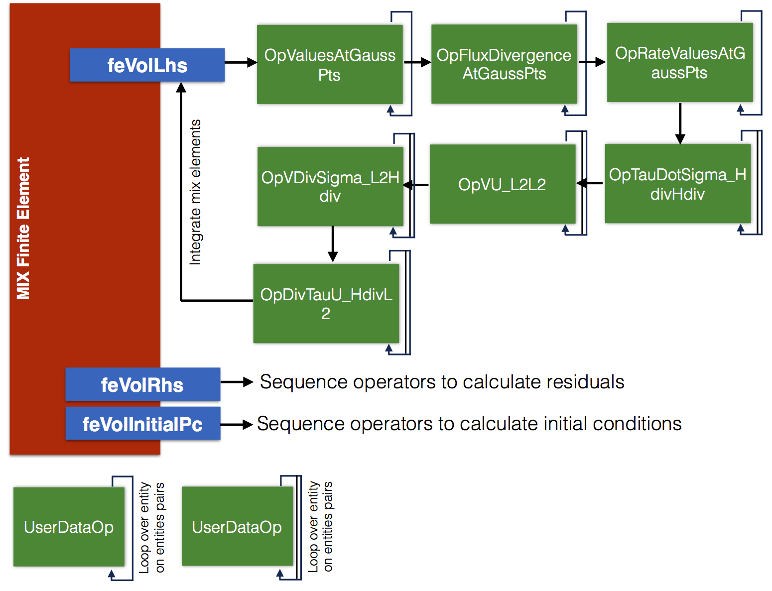
We have already discussed the last four operators in sequence for feVolLhs finite element instance, those are used to assemble tangent matrix blocks, i.e. \(\mathbf{C}\), \(\mathbf{G}\), \(\mathbf{H}\) and \(\mathbf{A}\). The first three operators are used to evaluate fields at integration points, i.e. capillary head, flux and rate of capillary head. Note that the first three operators have been reused from other tutorials.
In this problem, we use two generic implementations of finite element, MoFEM::VolumeElementForcesAndSourcesCore and MoFEM::FaceElementForcesAndSourcesCore, for integrating fields on volumes and faces. Finite element instances are iterated over a particular element in the problem, and for each entity on finite element entity, the sequence of UDO is called.
We use smart pointers to create the finite element instances, which gives the code flexibility and a safe memory management. The finite element instances are created in method MixTransport::UnsaturatedFlowElement::setFiniteElements as follows
Next, we set the integration rule, as has been discussed in tutorial COR-2: Solving the Poisson equation as follows
In addition, we add hooks to functions which are run at the beginning and the end of the loop over a particular element. Those functions are used to preprocess and postprocess the matrix assembly. Those pre-processing and post-processing hooks are added as follows
We use classes MixTransport::UnsaturatedFlowElement::preProcessVol and MixTransport::UnsaturatedFlowElement::postProcessVol to enforce essential boundary conditions. The method of enforcing essential boundary conditions is discussed in COR-0: Mixed formulation and integration on skeleton (h-adaptivity). In addition, in function MixTransport::UnsaturatedFlowElement::postProcessVol::operator()(), we scatter the vector of rate of capillary pressure on the field data. Since the rate of capillary head is not primary unknown but linear function of solution at current and previous steps, it is evaluated by PETSc for particular integration scheme.
Time solver provides vector of DOFs, \(\left(\frac{\textrm{d}\mathbf{p}}{\textrm{d}t}\right)^{i+1}_{n+1}\) at integration \(i+1\) and time step \(n+1\), and the above code scatters the vector values on the mesh, such that values of capillary head at integration points are evaluated early, i.e. \(\frac{\textrm{d}h}{\textrm{d}t}|^{i+1}_{n+1}\). Capillary head DOFs are sub-vectors of fePtr->ts_u_t.
The user data operators are added to the finite element calculating tangent matrix as follows
and similarly for other elements, evaluating the boundary conditions and the vector of residuals. For more details we refer to tutorial FUN-0: Hello world.
In addition, finite element instances are created to post-process results and to run time stepping monitor, see code in MixTransport::UnsaturatedFlowElement::setFiniteElements.
Once we have created finite element instances, in MixTransport::UnsaturatedFlowElement::setFiniteElements, we add finite instances to DM manager, such that the system of equations could be assembled. This is simply done by
Those functions are specific to MoFEM implementation, they have been implemented based on PETSc documentation, link, see Chapter 6.
Finally, we can solve the problem by creating TS solver and link it to DM as follows
Note that TS calls the finite elements instance by DM, similarly how SNES (Newton solver) calls finite elements in COR-5: A nonlinear Poisson equation, or KSP (Krylov solver) calls finite elements in COR-2: Solving the Poisson equation. The above is implemented in MixTransport::UnsaturatedFlowElement::solveProblem, where prior to solution, initial conditions are calculated, and statistics at the end printed to the terminal.
Application code is unsaturated_transport.cpp, which calls sequence of functions
Add example with hp-adaptivity
Implement block-solver and multigrid
Apply Kirchhoff transform
Add boundary condition for evaporation
Add air phase and mechanical filed
Add diffusion and other physical phenomena
Make example with flux history or head history. That is implemented but no example is added
Add diffusion and other physical phenomenas
