- Note
- Prerequisites of this tutorial include MSH-1: Create a 2D mesh from Gmsh and SCL-1: Poisson's equation (homogeneous BC)
-
High order geometry and schurs complement are present in the current code but outside the scope of this tutorial refer to ADV-0: Plastic problem
- Note
- Intended learning outcome:
- general structure of a program developed using MoFEM
- idea of Simple Interface in MoFEM and how to use it
- implementing vector valued problems like linear elasticity
- implementing boundary conditions specified on the part of the boundary
- developing code that can be compiled for 2D or 3D cases
- use of default forms integrators
- pushing UDOs to the Pipeline
- utilisation of tools to convert outputs (MOAB) and visualise them (Paraview)
The solution of the linear elasticity problem is presented in this tutorial. Lets consider an isotropic elastic cantilever beam with prescribed gravity load as presented in Figure 1.
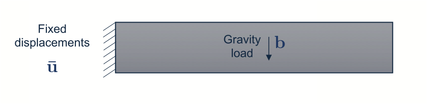
Figure 1: Cantilever beam considered in this example.
Strong form
In order to compute displacement vector field \(\mathbf{u}\), every point in the beam has to satisfy balance of linear momentum and boundary conditions as follows:
\[ \begin{align} \label{eq:momentum_balance} \begin{cases} \nabla \cdot \boldsymbol \sigma \left(\mathbf u(\mathbf{x}) \right) + \mathbf b =0 & \text { in } \Omega \\ \mathbf u(\mathbf{x}) = \bar{\mathbf{u}} & \text { on } \partial\Omega^\mathbf{u} \\ \boldsymbol \sigma \cdot \mathbf n = \bar {\mathbf t} & \text { on } \partial\Omega^\mathbf{t} \end{cases} \end{align} \]
where \(\mathbf{b}\) are body forces, \( \bar{\mathbf{u}} \) are fixed displacements, \( \bar{\mathbf{t}} \) is traction vector and \(\mathbf{n}\) is the unit normal vector on the boundary and \( \boldsymbol \sigma \) is the Cauchy stress tensor. In case of linear elasticity, small strains are assumed whereby the stress measure is defined as:
\[ \begin{align} \boldsymbol \sigma =& \mathbb D : \frac{1}{2} (\nabla \mathbf u^\text{T} + \nabla \mathbf u) \end{align} \]
where \( \mathbb D \) is the 4th order elasticity tensor.
Discretisation
Following a standard Galerkin approach as in SCL-1: Poisson's equation (homogeneous BC), the governing equations are discretised into weak form as follows:
\[ \begin{align} \int_{\Omega} \nabla \delta \mathbf u : \boldsymbol \sigma(\mathbf u) \, \mathrm d \Omega= - \int_{\Omega} \delta \mathbf u \cdot \mathbf b \, \mathrm d \Omega + \int_{\partial{\Omega}^\mathbf t} \delta \mathbf u \cdot \bar{\mathbf t} \, \mathrm d S \quad \forall\, \delta \mathbf u \in \mathbf{H}^1_0(\Omega) \end{align} \]
To approximate displacements \( \mathbf u\) and variance of displacements \( \delta \mathbf u\), once again we will use MoFEM's hierarchical shape functions:
\[ \begin{align} \mathbf u \approx \mathbf u^{h}=\sum_{j=0}^{N-1} \phi_{j} \bar{\mathbf{u}}_{j}, \quad \quad \delta \mathbf u \approx \delta \mathbf u^{h}=\sum_{j=0}^{N-1} \phi_{j} \delta \bar{\mathbf{u}}_{j} \end{align} \]
By substituting the above definitions into the weak form, the global system \( \mathbf{K U}=\mathbf{F}\) can be assembled, where elements contributions from every finite elements are computed as follows:
\[ \begin{align} \mathbf K_{i j}^{e}&=\int_{\Omega^{e}} \nabla \phi_{i} \mathbb D \nabla \phi_{j} \, \mathrm d \Omega \\ \mathbf F_{i}^{e}&=\int_{\partial \Omega^{e}} \phi_{i} \mathbf t \, \mathrm d S + \int_{\Omega^{e}} \phi_{i} \mathbf b \, \mathrm d \Omega \end{align} \]
The Gauss quadrature is utilised to calculate the integrals.
Implementation
In this section we will focus on the procedure to setup and solve vector-valued problems such as elasticity in MoFEM using MoFEM::Simple and Form Integrators, which are template UDOs used for common operations.
The code developed for this example can be compiled for both 2D and 3D cases by assigning the input parameter EXECUTABLE_DIMENSION in the CMakeFiles.txt prior to compilation and is used throughout the code to define the constant variable SPACE_DIM which is used as a template paramenter to assign the dimension of the executable:
Based on SPACE_DIM appropriate element types are defined in the following snippet for example, DomainEle in 2D are defined as faces while in 3D they are defined as volumes:
The main program then consists of a series of functions when invoking the function Example::runProblem():
where Example::readMesh() executes the mesh reading procedure, refer to MSH-1: Create a 2D mesh from Gmsh and MSH-2: Create a 3D mesh from Gmsh for an introduction to mesh generation.
Problem setup
The first function, Example::setupProblem() is used to setup the problem and involves adding the displacement field U on the entities of the mesh and determine the base function space, base, field rank and base order. For this problem We are adding displacement field U as both domain and a boundary field.
enum bases { AINSWORTH, DEMKOWICZ, LASBASETOPT };
const char *list_bases[LASBASETOPT] = {"ainsworth", "demkowicz"};
PetscInt choice_base_value = AINSWORTH;
LASBASETOPT, &choice_base_value, PETSC_NULL);
switch (choice_base_value) {
case AINSWORTH:
<< "Set AINSWORTH_LEGENDRE_BASE for displacements";
break;
case DEMKOWICZ:
<< "Set DEMKOWICZ_JACOBI_BASE for displacements";
break;
default:
break;
}
auto project_ho_geometry = [&]() {
Projection10NodeCoordsOnField ent_method(
mField,
"GEOMETRY");
};
PETSC_NULL);
} else {
}
auto no_rule = [](
int,
int,
int) {
return -1; };
field_eval_fe_ptr->getRuleHook = no_rule;
field_eval_fe_ptr->getOpPtrVector().push_back(
}
}
The space selected for displacement field U is H1 and dimension is SPACE_DIM that corresponds to a vector field with SPACE_DIM number of coefficients. Additionally, we define command line parameters -base and -order that specify the base and order of our base respectively with AINSWORTH_LEGENDRE_BASE and 2nd order selected by default.
Essential boundary conditions
The next function, Example::boundaryCondition() is used to apply homogeneous Dirichlet boundary conditions for our problem by utilise MoFEM's utility to remove degrees of freedom from a problem through the BcManager interface.
CHKERR bc_mng->removeBlockDOFsOnEntities(
simple->getProblemName(),
"REMOVE_X",
"U", 0, 0);
CHKERR bc_mng->removeBlockDOFsOnEntities(
simple->getProblemName(),
"REMOVE_Y",
"U", 1, 1);
CHKERR bc_mng->removeBlockDOFsOnEntities(
simple->getProblemName(),
"REMOVE_Z",
"U", 2, 2);
CHKERR bc_mng->removeBlockDOFsOnEntities(
simple->getProblemName(),
"REMOVE_ALL", "U", 0, 3);
CHKERR bc_mng->pushMarkDOFsOnEntities<DisplacementCubitBcData>(
simple->getProblemName(),
"U");
CHKERR bc_mng->addBlockDOFsToMPCs(
simple->getProblemName(),
"U");
}
For the examples considered in this tutorial, the provided meshes contain only one meshset FIX_ALL that will essentially fix displacements in all directions to zero. In Figure 2 we show selected triangles on the face of triangles that are used to define the FIX_ALL meshset. While for the 2D case, we select edge elements instead.
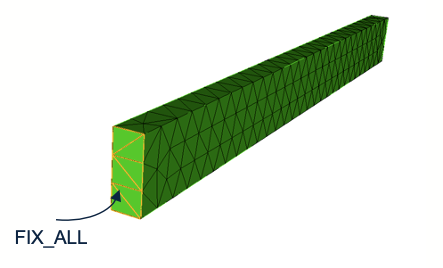
Figure 2: FIX_ALL block meshset specified on the mesh of the cantilever for 3D case.
Pushing operators to pipeline
The next function of the main program, Example::assembleSystem() is responsible for defining pipelines used to evaluate linear and bilinear forms of the system (refer to User data operators table) and assembly of the global matrices and vectors.
};
};
CHKERR pip->setBoundaryRhsIntegrationRule(integration_rule_bc);
CHKERR pip->setBoundaryLhsIntegrationRule(integration_rule_bc);
pip->getOpDomainLhsPipeline(), {H1}, "GEOMETRY");
pip->getOpDomainRhsPipeline(), {H1}, "GEOMETRY");
pip->getOpBoundaryRhsPipeline(), {NOSPACE}, "GEOMETRY");
pip->getOpBoundaryLhsPipeline(), {NOSPACE}, "GEOMETRY");
auto mat_D_ptr = boost::make_shared<MatrixDouble>();
mat_D_ptr, Sev::verbose);
pip->getOpDomainLhsPipeline().push_back(
new OpK(
"U",
"U", mat_D_ptr));
auto mat_grad_ptr = boost::make_shared<MatrixDouble>();
auto mat_strain_ptr = boost::make_shared<MatrixDouble>();
auto mat_stress_ptr = boost::make_shared<MatrixDouble>();
pip->getOpDomainRhsPipeline().push_back(
mat_grad_ptr));
mat_D_ptr, Sev::inform);
pip->getOpDomainRhsPipeline().push_back(
new OpSymmetrizeTensor<SPACE_DIM>(mat_grad_ptr, mat_strain_ptr));
pip->getOpDomainRhsPipeline().push_back(
new OpTensorTimesSymmetricTensor<SPACE_DIM, SPACE_DIM>(
mat_strain_ptr, mat_stress_ptr, mat_D_ptr));
pip->getOpDomainRhsPipeline().push_back(
[](double, double, double) constexpr { return -1; }));
pip->getOpDomainRhsPipeline(),
mField,
"U", Sev::inform);
pip->getOpBoundaryRhsPipeline(),
mField,
"U", -1, Sev::inform);
pip->getOpBoundaryLhsPipeline(),
mField,
"U", Sev::verbose);
}
Integration rule
The first part of this function, sets and pushes the integration rule for the finite element method to the pipeline.
};
};
CHKERR pip->setBoundaryRhsIntegrationRule(integration_rule_bc);
CHKERR pip->setBoundaryLhsIntegrationRule(integration_rule_bc);
Pushing domain stiffness matrix
The second part of this function, first calculates the local elasticity tensor through addMatBlockOps function depending on the MAT_ELASTIC block defined in the mesh file, then pushes the LHS stiffness matrix using alias OpK to the LHS pipeline.
auto mat_D_ptr = boost::make_shared<MatrixDouble>();
mat_D_ptr, Sev::verbose);
pip->getOpDomainLhsPipeline().push_back(
new OpK(
"U",
"U", mat_D_ptr));
The local elasticty tensor \( \mathbb D\) is calculate using the formula below:
\[ \begin{align} \mathbb D_{ijkl} = G \left[ \delta_{ik} \delta_{jl} + \delta_{il} \delta_{jk} \right] + A (K - \frac{2}{3} G) \left[ \delta_{ij} \delta_{kl} \right] \end{align} \]
where \( K\) and \( G\) are bulk and shear modulus, respectively. The coefficient \( A\) depends on the dimension of the problem, for 3D cases and plane strain formulation it is simply \( A = 1\), whereas for plane stress it takes the following form:
\[ \begin{align} A=\frac{2 G}{K+\frac{4}{3} G} \end{align} \]
Using the FTensor::Index type these formulas can be directly implemented using Einstein's summation convention as shown below, within the Example::addMatBlockOps() function:
auto set_material_stiffness = [&]() {
}
auto t_D = getFTensor4DdgFromMat<SPACE_DIM, SPACE_DIM, 0>(*mat_D_ptr);
};
- Note
- Note that depending on SPACE_DIM our code will appropriately sum over all the indices and set coefficient \( A \) for plane stress or 3D case.
The operator OpK integrates the bilinear form:
\[ \begin{align} \mathbf K^e_{ij} = \int_{\Omega^e} \nabla \phi_i \mathbb D \nabla \phi_j \, \mathrm d \Omega \end{align} \]
and subsequently assembles it into global system matrix \( \mathbf K \). Note that once again, a new operator does not have to be defined as OpK is simply an alias to existing operator from MoFEM's repertoire. To that operator we are passing previously defined container that stores elasticity tensor \( \mathbb D \).
I>::OpGradSymTensorGrad<BASE_DIM, SPACE_DIM, SPACE_DIM, 0>;
The utilised OpGradSymTensorGrad form integrator template of Bilinear Form has four parameters: rank of the base, rank of row field, rank of the column field and finally, the increment of elasticity tensor, which in case of homogeneous material can be set to 0.
More info about available Form Integrators can be found in User data operators table.
Pushing internal forces
The next part of the Example::assembleSystem() function calculates the internal forces for the system which is required to enforce the boundary conditions (defined as \( \mathbf K \mathbf u_e \) refer to SCL-1: Poisson's equation (homogeneous BC) for an in depth description). For elastic problems, this requires calculating the displacement gradient \( \nabla \mathbf u \), strain \( \boldsymbol \varepsilon \) and stress \( \boldsymbol \sigma \) of the system by pushing the relevant operatiors to the RHS pipeline.
auto mat_grad_ptr = boost::make_shared<MatrixDouble>();
auto mat_strain_ptr = boost::make_shared<MatrixDouble>();
auto mat_stress_ptr = boost::make_shared<MatrixDouble>();
pip->getOpDomainRhsPipeline().push_back(
mat_grad_ptr));
mat_D_ptr, Sev::inform);
pip->getOpDomainRhsPipeline().push_back(
new OpSymmetrizeTensor<SPACE_DIM>(mat_grad_ptr, mat_strain_ptr));
pip->getOpDomainRhsPipeline().push_back(
new OpTensorTimesSymmetricTensor<SPACE_DIM, SPACE_DIM>(
mat_strain_ptr, mat_stress_ptr, mat_D_ptr));
pip->getOpDomainRhsPipeline().push_back(
[](double, double, double) constexpr { return -1; }));
This is achieved by pushing a series of operators as follows:
OpCalculateVectorFieldGradient computes the gradient of the displacement field \( \nabla \mathbf u^{h}=\sum_{m=0}^{N-1} \nabla \phi_m \bar{\mathbf u}_m \)OpSymmetrizeTensor symmetrises the previously computed gradient to compute small strain tensor \( \boldsymbol \varepsilon = \frac{1}{2} (\nabla \mathbf u^\text{T} + \nabla \mathbf u) \)OpTensorTimesSymmetricTensor is another form integrator that computes Cauchy stress: \( \boldsymbol \sigma = \mathbb D : \boldsymbol \varepsilon \)OpInternalForce is an alias of the FormsIntegrators OpGradTimesSymTensor which computes \( (\mathbf K \mathbf u_e)_j = \nabla \phi_i \mathbf \sigma_{ij} \)
Natural boundary conditions
For natural boundary conditions we will only specify simple gravity load on the entire domain. We have to push into our Domain RHS pipeline an operator that calculates the following integral:
\[ \begin{align} \mathbf F_{i}^{e}&=\int_{\Omega^{e}} \phi_{i} \mathbf b \, \mathrm d V \end{align} \]
This operation can be done by utilsing the DomanRhsBc::AddFluxToPipeline alias which applies a flux User Data Operator into RHS pipeline as shown below.
pip->getOpBoundaryRhsPipeline(), mField, "U", -1, Sev::inform);
pip->getOpBoundaryLhsPipeline(), mField, "U", Sev::verbose);
Solver setup
With appropriately defined pipelines for assembling the global system of equations \( \mathbf{K} \mathbf{U} = \mathbf{F} \), the next functions Example::solveSystem() sets up PETSc solver and calculates it directly or iteratively based on specified settings.
CHKERR KSPSetFromOptions(solver);
auto set_essential_bc = [&]() {
auto pre_proc_rhs = boost::make_shared<FEMethod>();
auto post_proc_rhs = boost::make_shared<FEMethod>();
auto post_proc_lhs = boost::make_shared<FEMethod>();
auto get_pre_proc_hook = [&]() {
return EssentialPreProc<DisplacementCubitBcData>(
mField, pre_proc_rhs,
{});
};
pre_proc_rhs->preProcessHook = get_pre_proc_hook();
auto get_post_proc_hook_rhs = [this, post_proc_rhs]() {
CHKERR EssentialPostProcRhs<DisplacementCubitBcData>(
mField,
post_proc_rhs, 1.)();
CHKERR EssentialPostProcRhs<MPCsType>(
mField, post_proc_rhs, 1.)();
};
auto get_post_proc_hook_lhs = [this, post_proc_lhs]() {
CHKERR EssentialPostProcLhs<DisplacementCubitBcData>(
mField,
post_proc_lhs, 1.)();
CHKERR EssentialPostProcLhs<MPCsType>(
mField, post_proc_lhs)();
};
post_proc_rhs->postProcessHook = get_post_proc_hook_rhs;
post_proc_lhs->postProcessHook = get_post_proc_hook_lhs;
ksp_ctx_ptr->getPreProcComputeRhs().push_front(pre_proc_rhs);
ksp_ctx_ptr->getPostProcComputeRhs().push_back(post_proc_rhs);
ksp_ctx_ptr->getPostProcSetOperators().push_back(post_proc_lhs);
};
auto setup_and_solve = [&]() {
BOOST_LOG_SCOPED_THREAD_ATTR("Timeline", attrs::timer());
MOFEM_LOG(
"TIMER", Sev::inform) <<
"KSPSetUp";
MOFEM_LOG(
"TIMER", Sev::inform) <<
"KSPSetUp <= Done";
MOFEM_LOG(
"TIMER", Sev::inform) <<
"KSPSolve";
MOFEM_LOG(
"TIMER", Sev::inform) <<
"KSPSolve <= Done";
};
CHKERR schur_ptr->setUp(solver);
} else {
}
CHKERR VecGhostUpdateBegin(
D, INSERT_VALUES, SCATTER_FORWARD);
CHKERR VecGhostUpdateEnd(
D, INSERT_VALUES, SCATTER_FORWARD);
} else {
}
<< "U_X: " << t_disp(0) << " U_Y: " << t_disp(1);
else
<< "U_X: " << t_disp(0) << " U_Y: " << t_disp(1)
<< " U_Z: " << t_disp(2);
}
}
}
Note that in case of simple linear problems like elasticity considered therein the above snippet will look very similar. A detailed description of each function can be found e.g. in SCL-1: Poisson's equation (homogeneous BC).
Postprocessing pipeline
Finally, once the solver calculations are completed and solution vector is obtained, it is necessary to save the data on the visualisation mesh and compute quantities of interest like strains and stresses. In function Example::outputResults() we will define pipeline to postprocess the results and save the calculated values to the output mesh.
auto det_ptr = boost::make_shared<VectorDouble>();
auto jac_ptr = boost::make_shared<MatrixDouble>();
auto inv_jac_ptr = boost::make_shared<MatrixDouble>();
pip->getDomainRhsFE().reset();
pip->getDomainLhsFE().reset();
pip->getBoundaryRhsFE().reset();
pip->getBoundaryLhsFE().reset();
auto post_proc_mesh = boost::make_shared<moab::Core>();
auto post_proc_begin = boost::make_shared<PostProcBrokenMeshInMoabBaseBegin>(
auto post_proc_end = boost::make_shared<PostProcBrokenMeshInMoabBaseEnd>(
auto calculate_stress_ops = [&](auto &pip) {
auto mat_grad_ptr = boost::make_shared<MatrixDouble>();
auto mat_strain_ptr = boost::make_shared<MatrixDouble>();
auto mat_stress_ptr = boost::make_shared<MatrixDouble>();
"U", mat_grad_ptr));
auto mat_D_ptr = boost::make_shared<MatrixDouble>();
pip.push_back(
new OpSymmetrizeTensor<SPACE_DIM>(mat_grad_ptr, mat_strain_ptr));
pip.push_back(new OpTensorTimesSymmetricTensor<SPACE_DIM, SPACE_DIM>(
mat_strain_ptr, mat_stress_ptr, mat_D_ptr));
auto u_ptr = boost::make_shared<MatrixDouble>();
pip.push_back(new OpCalculateVectorFieldValues<SPACE_DIM>("U", u_ptr));
auto x_ptr = boost::make_shared<MatrixDouble>();
pip.push_back(
new OpCalculateVectorFieldValues<SPACE_DIM>("GEOMETRY", x_ptr));
return boost::make_tuple(u_ptr, x_ptr, mat_strain_ptr, mat_stress_ptr);
};
auto get_tag_id_on_pmesh = [&](bool post_proc_skin)
{
int def_val_int = 0;
Tag tag_mat;
"MAT_ELASTIC", 1, MB_TYPE_INTEGER, tag_mat,
MB_TAG_CREAT | MB_TAG_SPARSE, &def_val_int);
auto meshset_vec_ptr =
std::regex((boost::format("%s(.*)") % "MAT_ELASTIC").str()));
std::unique_ptr<Skinner> skin_ptr;
if (post_proc_skin) {
auto boundary_meshset =
simple->getBoundaryMeshSet();
skin_ents, true);
}
for (
auto m : meshset_vec_ptr) {
true);
int const id =
m->getMeshsetId();
ents_3d = ents_3d.subset_by_dimension(
SPACE_DIM);
if (post_proc_skin) {
CHKERR skin_ptr->find_skin(0, ents_3d,
false, skin_faces);
ents_3d = intersect(skin_ents, skin_faces);
}
}
return tag_mat;
};
auto post_proc_domain = [&](auto post_proc_mesh) {
auto post_proc_fe =
boost::make_shared<PostProcEleDomain>(
mField, post_proc_mesh);
using OpPPMap = OpPostProcMapInMoab<SPACE_DIM, SPACE_DIM>;
auto [u_ptr, x_ptr, mat_strain_ptr, mat_stress_ptr] =
calculate_stress_ops(post_proc_fe->getOpPtrVector());
post_proc_fe->getOpPtrVector().push_back(
post_proc_fe->getPostProcMesh(), post_proc_fe->getMapGaussPts(),
{},
{{"U", u_ptr}, {"GEOMETRY", x_ptr}},
{},
{{"STRAIN", mat_strain_ptr}, {"STRESS", mat_stress_ptr}}
)
);
post_proc_fe->setTagsToTransfer({get_tag_id_on_pmesh(false)});
return post_proc_fe;
};
auto post_proc_boundary = [&](auto post_proc_mesh) {
auto post_proc_fe =
boost::make_shared<PostProcEleBdy>(mField, post_proc_mesh);
post_proc_fe->getOpPtrVector(), {}, "GEOMETRY");
auto op_loop_side =
auto [u_ptr, x_ptr, mat_strain_ptr, mat_stress_ptr] =
calculate_stress_ops(op_loop_side->getOpPtrVector());
post_proc_fe->getOpPtrVector().push_back(op_loop_side);
auto mat_traction_ptr = boost::make_shared<MatrixDouble>();
post_proc_fe->getOpPtrVector().push_back(
mat_traction_ptr));
using OpPPMap = OpPostProcMapInMoab<SPACE_DIM, SPACE_DIM>;
post_proc_fe->getOpPtrVector().push_back(
post_proc_fe->getPostProcMesh(), post_proc_fe->getMapGaussPts(),
{},
{{"U", u_ptr}, {"GEOMETRY", x_ptr}, {"T", mat_traction_ptr}},
{},
{{"STRAIN", mat_strain_ptr}, {"STRESS", mat_stress_ptr}}
)
);
post_proc_fe->setTagsToTransfer({get_tag_id_on_pmesh(true)});
return post_proc_fe;
};
PetscBool post_proc_skin_only = PETSC_FALSE;
post_proc_skin_only = PETSC_TRUE;
&post_proc_skin_only, PETSC_NULL);
}
if (post_proc_skin_only == PETSC_FALSE) {
pip->getDomainRhsFE() = post_proc_domain(post_proc_mesh);
} else {
pip->getBoundaryRhsFE() = post_proc_boundary(post_proc_mesh);
}
post_proc_begin->getFEMethod());
CHKERR pip->loopFiniteElements();
post_proc_end->getFEMethod());
CHKERR post_proc_end->writeFile(
"out_elastic.h5m");
}
We can reuse LHS domain pipeline, for the purpose of postprocessing. The following line resets (cleans) the operators pushed previously for each pipeline.
pip->getDomainRhsFE().reset();
pip->getDomainLhsFE().reset();
pip->getBoundaryRhsFE().reset();
pip->getBoundaryLhsFE().reset();
In the next few lines we create various postprocessing objects including the reference mesh and lists of elements to postprocess.
auto post_proc_mesh = boost::make_shared<moab::Core>();
auto post_proc_begin = boost::make_shared<PostProcBrokenMeshInMoabBaseBegin>(
mField, post_proc_mesh);
auto post_proc_end = boost::make_shared<PostProcBrokenMeshInMoabBaseEnd>(
mField, post_proc_mesh);
Then we define a series of functions including, calculate_stress_ops, post_proc_domain and post_proc_boundary which push the operators required to output the displacement \( \mathbf{u} \), current position \( \mathbf{x} \), strain \( \boldsymbol{\varepsilon} \) and stress \( \boldsymbol{\sigma} \) for the domain and boundary.
Running code and visualisation
In order to run the program that we have been discussing in this tutorial, you will do the following steps
- First, go to the directory where the binary file named
elastic is located. Depending on how you install MoFEM shown in this page Installation with Spack (Scripts), going to the directory would be something similar to this
- For user version installation
cd mofem_install/um_view/tutorials/vec-0/
- For developer version installation
cd mofem_install/mofem-cephas/mofem/users_modules/um-build-RelWithDebInfo-abcd1234/tutorials/vec-0
- Second, check the parameters in the param_file.petsc. These are PETSc parameters and you should only use parameters that are needed for a particular solver, in this case KSP solver. Only the following parameters should be uncommented
## Linear solver
-ksp_type fgmres
-pc_type lu
-pc_factor_mat_solver_type mumps
-ksp_monitor
- Third, in the terminal, run commands to partition the input mesh and start the analysis
./elastic_3d -file_name beam_3D.cub -
order 2
This will produce out_elastic.h5m file which we can convert using
mbconvert out_elastic.h5m out_elastic_3D.vtk
The file out_elastic_3D.vtk can be opened in Paraview. Using the filter WarpByVector allows to visualise the deformation as shown in Figure 3.
We can also compute 2D case of the beam. Following the same process as that for 3D with the commands:
./elastic_2d -file_name beam_2D.cub -
order 2
and generate vtk file using:
mbconvert out_elastic.h5m out_elastic_2D.vtk
Figure 3: Deformation of cantilever beams for 2D and 3D case. The color map represents displacements U.
Note that the beams, both for 2D and 3D cases experience spurious deformation at the free end. This is a known feature of small strain kinematic description. To mitigate this issue, a large strain geometrically nonlinear formulation can be used. The extension of the above tutorial to such nonlinear case can be found in VEC-2: Nonlinear elastic. We propose there a simple Hencky strain measure that improves the behaviour of the material experiencing large rotations.
Plain program
The full source code of the main program can be accessed below: elastic.cpp

