COR-10: Navier-Stokes equation

Table of Contents

• Introduction
• Non-dimensionalization and scaling
• Finite-element formulation
  • Weak form
  • Note on the choice of spaces for the mixed problem
• Implementation
  • Reading mesh and input parameters
  • Setting up fields, finite elements and the problem itself
  • Solving the problem and post-processing the results
• Running the example
  • Stokes equation
  • Navier-Stokes equations

Introduction

Navier-Stokes equations (NSE), governing the motion of a viscous fluid, are used in various applications: from simulations of the flow in blood vessels to studies of the air flow around aeroplane wings and rotor blades, scaling up to models of ocean and atmospheric currents. Even in the case of an incompressible steady flow, NSE are non-linear due to the effect of the inertia, which is more pronounced in case of a higher Reynolds number. In this tutorial we discuss the implementation of a viscous fluid model in MoFEM using hierarchical basis functions. This approach permits us to locally increase the order of approximation, enforcing conformity across finite element boundaries, without the need to change the implementation of an element. Moreover, the requirement of different approximation orders for primal (velocity) and dual (pressure) variables, necessary for a simulation of the flow using the mixed formulation, can be easily satisfied.

Problem statement

An incompressible isoviscous steady-state flow in a domain \(\Omega\) is governed by the following equations:

\[ \begin{align} \label{eq:balance_momentum} \rho \left(\mathbf{u}\cdot\nabla\right)\mathbf{u} - \mu\nabla^2\mathbf{u} + \nabla p &= \mathbf{f},\\ \label{eq:cont} \nabla\cdot\mathbf{u} &= 0, \end{align} \]

where \eqref{eq:balance_momentum} is the set of Navier-Stokes equations, representing the balance of the momentum, and \eqref{eq:cont} is the continuity equation; \(\mathbf{u}=[u_x, u_y, u_z]^\intercal\) is the velocity field, \(p\) is the hydrostatic pressure field, \(\rho\) is the fluid mass density, \(\mu\) is fluid viscosity and $\mathbf{f}$ is the density of external forces. The boundary value problem complements the above equations by the Dirichlet and Neumann conditions on the boundary \(\partial\Omega\):

\[ \begin{align} \label{eq:bc_d}\mathbf{u} = \mathbf{u}_D & \;\text{on}\; \Gamma_D,\\ \label{eq:bc_n}\mathbf{n}\cdot \left[-p\mathbf{I}+\mu\left(\nabla\mathbf{u} + \nabla\mathbf{u}^\intercal\right)\right] = \mathbf{g}_N & \;\text{on} \;\Gamma_N, \end{align} \]

where \(\mathbf{u}_D\) is the prescribed velocity on the part of the boundary \(\Gamma_D\subset\partial\Omega\), and \(\mathbf{g}_N\) is the prescribed traction vector on the part of the boundary \(\Gamma_N\subset\partial\Omega\), \(\mathbf{n}\) is an outward normal.

In this tutorial we will solve the problem of the fluid flow around a rigid sphere (see Figure 1) of a radius \(r\) positioned in the centre of a cubic domain, the side length \(2l\) of which is considered sufficiently large compared to \(r\), so that a uniform far-field velocity on the exterior boundaries is valid (note that the body forces are neglected). Exploiting the symmetry of the problem, we will use a quarter of the domain in our simulations.

Figure 1: (a) Finite-element mesh used for simulation of fluid flow around a rigid sphere. (b) Sketch of the problem set-up on a section $z=0$ of the mesh.

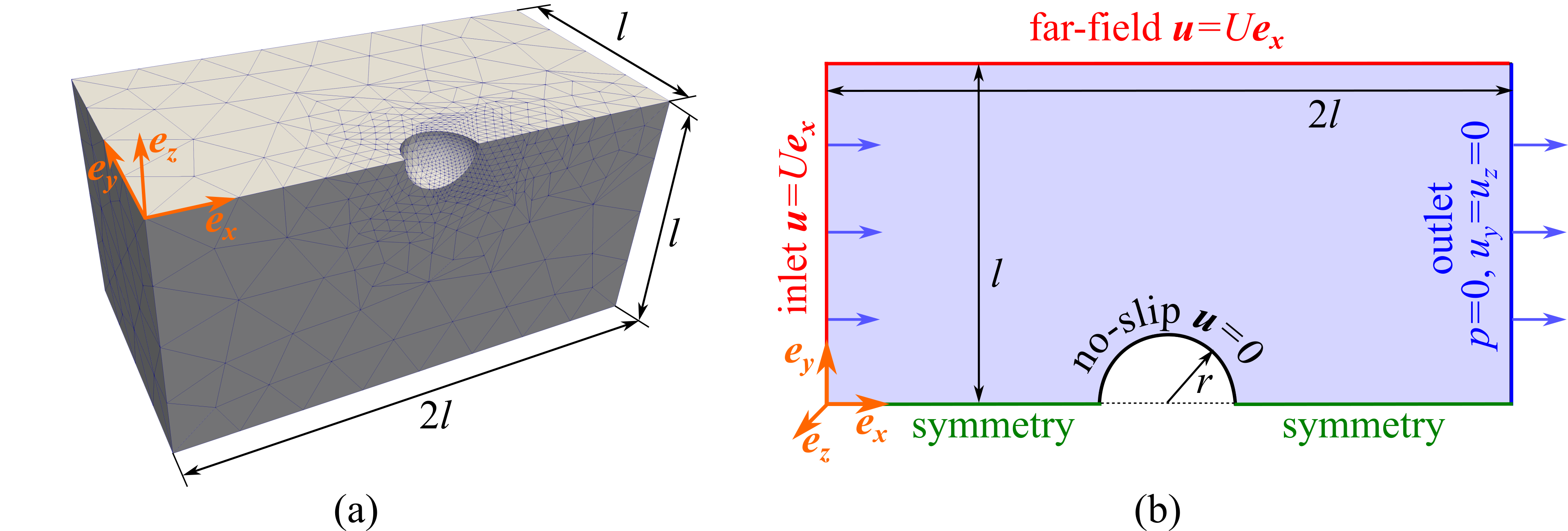
Note that due to the structure of differential operators in the Navier-Stokes equations \eqref{eq:balance_momentum}, the fluid pressure has to be specified on a part of boundary in order to obtain a unique solution. To achieve that, we will combine Dirichlet and Neumann condition on the outlet boundary of the domain, see see Figure 1. In the case when the flow is perpendicular to the boundary ( \(u_y = u_z = 0\)), which is enforced by the Dirichlet boundary condition, the hydrostatic fluid pressure equals to the normal traction on such boundary, see Theorem 1 in [10].

Non-dimensionalization and scaling

Reynolds number is introduced for the problems governed by the Navier-Stokes equations as a measure of the ratio of inertial forces to viscous forces:

\[ \begin{equation} \mathcal{R} = \frac{\rho U L }{\mu}, \end{equation} \]

where \(U\) is the scale for the velocity and \(L\) is a relevant length scale. For the problem of the fluid flow around a sphere, considered in this tutorial, the far-field velocity plays the role of the velocity scale, while \(L=2r\), where \(r\) is the radius of the sphere.

When viscous forces dominate over the inertia forces, \(\mathcal{R} \ll 1\), the non-linear term in \eqref{eq:balance_momentum} can be neglected, simplifying NSE down to Stokes equations. However, often this is not the case, i.e. the nonlinear term may become dominant over the viscous forces. In these cases non-dimensionalization (scaling) of Navier-Stokes equations is very useful, which permits to decrease the number of coefficients to only one – Reynolds number \(\mathcal{R}\). The following scales can be used for the case of flow with relatively low Reynolds number (e.g. less than 100).

Non-dimensionalization of Navier-Stokes equations

Physical quantity	Scale	Dimensionless variable
Length	\(L\)	\(\mathbf{x}^{*}=\mathbf{x}\:/\:L, \quad \nabla^{*}(\cdot) = L\nabla(\cdot)\)
Velocity	\(U\)	\(\mathbf{u}^{*}=\mathbf{u}\:/\:U\)
Pressure	\(P=\frac{\mu U}{L}\)	\(p^{*}=p\:/\:P\)

Mote that the scale for pressure depends on the scales for the length and the velocity. Using these scales, Navier-stokes equations (1) - (2) can be written in the following dimensionless form (considering zero external forces):

\[ \begin{align} \label{eq:balance_momentum_dim_less} \mathcal{R} \left(\mathbf{u}^{*}\cdot\nabla^{*}\right)\mathbf{u}^{*} - (\nabla^{*})^2\mathbf{u}^{*} + \nabla^{*} p^{*} &= 0,\\ \label{eq:cont_dim_less} \nabla^{*}\cdot\mathbf{u}^{*} &= 0, \end{align} \]

Note that now the influence of the non-linearity (inertia terms) on the problem is fully controlled by the value of the Reynolds number. On the one hand, if \(\mathcal{R} \ll 1\), or if one simply wants to consider the Stokes equation, the nonlinear term can be dropped. On the other hand, if the Reynolds number is sufficiently high, then the non-linearity can become strong and may pose problems for convergence (see below discussion of the linearisation of the problem for the Newton-Raphson method). In this case a certain iterative procedure can be used to obtain a solution. Indeed, to find the solution for a given Reynolds number, a number of intermediate problems can be solved for range of smaller \(\mathcal{R}\), eventually reaching the original value. Such technique will also be used in this tutorial. Note also that below we will drop the * symbol, implying that during computation all considered quantities are dimensionless, and a transformation to the dimensional variables is performed before post-processing of the results takes place.

Finite-element formulation

Weak form

The weak statement of the problem \eqref{eq:balance_momentum}-\eqref{eq:bc_n} reads: Find a vector field \(\mathbf{u} \in \mathbf{H}^1(\Omega)\) and a scalar field \(p \in L^2(\Omega)\), such that for any test functions \(\mathbf{v} \in \mathbf{H}^1_0(\Omega)\) and \(q \in L^2(\Omega)\):

\[ \begin{align} \label{eq:weak} \mathcal{R}\int\limits_\Omega \left(\mathbf{u}\cdot\nabla\right)\mathbf{u} \cdot\mathbf{v} \,d\Omega + \int\limits_{\Omega}\nabla\mathbf{u}\mathbin{:}\nabla\mathbf{v}\, d\Omega - \int\limits_{\Omega}p\, \nabla\cdot\mathbf{v} \, d\Omega &= \int\limits_{\Omega}\mathbf{f}\cdot\mathbf{v}\,d\Omega + \int\limits_{\Gamma_N}\mathbf{g}_N\cdot\mathbf{v}\,d\Gamma_N,\\ - \int\limits_{\Omega}q\, \nabla\cdot\mathbf{u} \, d\Omega &= 0 \end{align} \]

Upon finite-element discretization of the domain \(\Omega\), we consider interpolation of both unknown fields introducing shape functions on each element: \begin{equation} \label{eq:shape} u_i = \sum\limits_{\alpha=1}^{n_{\mathbf{u}}} N_{\alpha}\, u_i^\alpha, \quad p = \sum\limits_{\beta=1}^{n_p} \Phi_{\beta}\, p^\beta; \quad v_i = \sum\limits_{\alpha=1}^{n_{\mathbf{u}}} N_{\alpha}\, v_i^\alpha, \quad q = \sum\limits_{\beta=1}^{n_p} \Phi_{\beta}\, q^\beta, \end{equation} where \(n_{\mathbf{u}}\) is the number of shape functions associated with the velocity field, and $n_p$ is the similar number for the pressure field. Using the hierarchical basis approximation, the vector of the shape functions can be decomposed into four sub-vectors, consisting of shape functions associated with element's entities: vertices, edges, faces and the volume of the element, e.g. for the velocity field:

\[ \begin{equation} \label{eq:shape_hier} \mathbf{N}^\textit{el} = \left[N_1, \ldots N_\alpha, \ldots N_{n_{\mathbf{u}}}\right]^\intercal = \left[\mathbf{N}^\textit{ver}, \mathbf{N}^\textit{edge}, \mathbf{N}^\textit{face}, \mathbf{N}^\textit{vol}\right]^\intercal. \end{equation} \]

Note on the choice of spaces for the mixed problem

Note that in the weak statement velocity and pressure fields belong to different spaces: \(H^1\) and \(L^2\), respectively. Two different approaches can be used for implementing such mixed formulation in the finite-element framework. One can use generalised Taylor-Hood elements, which feature continuous ( \(H^1\) ) approximation of both velocity and pressure fields, however, in order to enforce stability, the approximations functions for the pressure field should be one order lower than those for the velocity field. Furthermore, Taylor-Hood elements impose certain constraints on the mesh, see [52]. Alternatively, a discontinuous approximation for pressure can be used, however, in this case the difference between the orders of approximation functions for velocity and for pressure should be 2.

Implementation

The example class has necessary fields to store input parameters and internal data structures, as well as a set of functions for setting up and solving the problem:

struct NavierStokesExample {
 
  NavierStokesExample(MoFEM::Interface &m_field) : mField(m_field) {
    commonData = boost::make_shared<NavierStokesElement::CommonData>(m_field);
  }
  ~NavierStokesExample() {
    CHKERR SNESDestroy(&snes);
    CHKERR DMDestroy(&dM);
  }
 
  MoFEMErrorCode runProblem();
 
private:
  MoFEM::Interface &mField;
 
  PetscBool isPartitioned = PETSC_FALSE;
 
  int orderVelocity = 2; // default approximation orderVelocity
  int orderPressure = 1; // default approximation orderPressure
  int numHoLevels = 0;
  PetscBool isDiscontPressure = PETSC_FALSE;
  PetscBool isHoGeometry = PETSC_TRUE;
 
  double pressureScale = 1.0;
  double lengthScale = 1.0;
  double velocityScale = 1.0;
  double reNumber = 1.0;
  double density;
  double viscosity;
  PetscBool isStokesFlow = PETSC_FALSE;
 
  int numSteps = 1;
  double lambdaStep = 1.0;
  double lambda = 0.0;
  int step;
 
  Range solidFaces;
  BitRefLevel bitLevel;
 
  DM dM;
  SNES snes;
 
  boost::shared_ptr<NavierStokesElement::CommonData> commonData;
 
  SmartPetscObj<Vec> D;
  SmartPetscObj<Vec> F;
  SmartPetscObj<Mat> Aij;
 
  boost::shared_ptr<VolumeElementForcesAndSourcesCore> feLhsPtr;
  boost::shared_ptr<VolumeElementForcesAndSourcesCore> feRhsPtr;
 
  boost::shared_ptr<FaceElementForcesAndSourcesCore> feDragPtr;
  boost::shared_ptr<VolumeElementForcesAndSourcesCoreOnSide> feDragSidePtr;
 
  boost::shared_ptr<DirichletDisplacementBc> dirichletBcPtr;
  boost::ptr_map<std::string, NeumannForcesSurface> neumannForces;
 
  boost::shared_ptr<PostProcVol> fePostProcPtr;
  boost::shared_ptr<PostProcFace> fePostProcDragPtr;
 
  MoFEMErrorCode readInput();
  MoFEMErrorCode findBlocks();
  MoFEMErrorCode setupFields();
  MoFEMErrorCode defineFiniteElements();
  MoFEMErrorCode setupDiscreteManager();
  MoFEMErrorCode setupAlgebraicStructures();
  MoFEMErrorCode setupElementInstances();
  MoFEMErrorCode setupSNES();
  MoFEMErrorCode solveProblem();
  MoFEMErrorCode postProcess();
};

The set of functions used in this tutorials in the following:

MoFEMErrorCode NavierStokesExample::runProblem() {
  MoFEMFunctionBegin;
  CHKERR readInput();
  CHKERR findBlocks();
  CHKERR setupFields();
  CHKERR defineFiniteElements();
  CHKERR setupDiscreteManager();
  CHKERR setupAlgebraicStructures();
  CHKERR setupElementInstances();
  CHKERR setupSNES();
  CHKERR solveProblem();
  MoFEMFunctionReturn(0);
}

The function ExampleNavierStokes::runProblem is executed from the main function:

int main(int argc, char *argv[]) {
 
  const char param_file[] = "param_file.petsc";
  // Initialise MoFEM
  MoFEM::Core::Initialize(&argc, &argv, param_file, help);
 
  try {
 
    // Create mesh database
    moab::Core mb_instance;              // create database
    moab::Interface &moab = mb_instance; // create interface to database
 
    // Create MoFEM database and link it to MoAB
    MoFEM::Core core(moab);
    MoFEM::Interface &m_field = core;
 
    NavierStokesExample ex(m_field);
    CHKERR ex.runProblem();
  }
  CATCH_ERRORS;
 
  // finish work cleaning memory, getting statistics, etc
  MoFEM::Core::Finalize();
  return 0;
}

Reading mesh and input parameters

The workflow of solving a problem using the finite-element method starts from reading the mesh and other input parameters:

MoFEMErrorCode NavierStokesExample::readInput() {
  MoFEMFunctionBegin;
  char mesh_file_name[255];
  PetscBool flg_mesh_file;
 
  CHKERR PetscOptionsBegin(PETSC_COMM_WORLD, "", "NAVIER_STOKES problem",
                           "none");
 
  CHKERR PetscOptionsString("-my_file", "mesh file name", "", "mesh.h5m",
                            mesh_file_name, 255, &flg_mesh_file);
  CHKERR PetscOptionsBool("-my_is_partitioned", "is partitioned?", "",
                          isPartitioned, &isPartitioned, PETSC_NULL);
 
  CHKERR PetscOptionsInt("-my_order_u", "approximation orderVelocity", "",
                         orderVelocity, &orderVelocity, PETSC_NULL);
  CHKERR PetscOptionsInt("-my_order_p", "approximation orderPressure", "",
                         orderPressure, &orderPressure, PETSC_NULL);
  CHKERR PetscOptionsInt("-my_num_ho_levels",
                         "number of higher order boundary levels", "",
                         numHoLevels, &numHoLevels, PETSC_NULL);
  CHKERR PetscOptionsBool("-my_discont_pressure", "discontinuous pressure", "",
                          isDiscontPressure, &isDiscontPressure, PETSC_NULL);
  CHKERR PetscOptionsBool("-my_ho_geometry", "use second order geometry", "",
                          isHoGeometry, &isHoGeometry, PETSC_NULL);
 
  CHKERR PetscOptionsScalar("-my_length_scale", "length scale", "", lengthScale,
                            &lengthScale, PETSC_NULL);
  CHKERR PetscOptionsScalar("-my_velocity_scale", "velocity scale", "",
                            velocityScale, &velocityScale, PETSC_NULL);
  CHKERR PetscOptionsBool("-my_stokes_flow", "stokes flow", "", isStokesFlow,
                          &isStokesFlow, PETSC_NULL);
 
  CHKERR PetscOptionsInt("-my_step_num", "number of steps", "", numSteps,
                         &numSteps, PETSC_NULL);
 
  ierr = PetscOptionsEnd();
 
  if (flg_mesh_file != PETSC_TRUE) {
    SETERRQ(PETSC_COMM_SELF, 1, "*** ERROR -my_file (MESH FILE NEEDED)");
  }
 
  // Read whole mesh or part of it if partitioned
  if (isPartitioned == PETSC_TRUE) {
    // This is a case of distributed mesh and algebra. In that case each
    // processor keeps only part of the problem.
    const char *option;
    option = "PARALLEL=READ_PART;"
             "PARALLEL_RESOLVE_SHARED_ENTS;"
             "PARTITION=PARALLEL_PARTITION;";
    CHKERR mField.get_moab().load_file(mesh_file_name, 0, option);
  } else {
    // In this case, we have distributed algebra, i.e. assembly of vectors and
    // matrices is in parallel, but whole mesh is stored on all processors.
    // snes and matrix scales well, however problem set-up of problem is
    // not fully parallel.
    const char *option;
    option = "";
    CHKERR mField.get_moab().load_file(mesh_file_name, 0, option);
  }
  CHKERR mField.rebuild_database();
 
  bitLevel.set(0);
  CHKERR mField.getInterface<BitRefManager>()->setBitRefLevelByDim(0, 3,
                                                                   bitLevel);
 
  MoFEMFunctionReturn(0);
}

Once the mesh is read, we find the set of tetrahedra corresponding to the computational domain. Furthermore, we identify the fluid-structure interface, i.e. the set of triangles corresponding to the surface of the sphere:

MoFEMErrorCode NavierStokesExample::findBlocks() {
  MoFEMFunctionBegin;
 
  for (_IT_CUBITMESHSETS_BY_SET_TYPE_FOR_LOOP_(mField, BLOCKSET, bit)) {
    if (bit->getName().compare(0, 9, "MAT_FLUID") == 0) {
      const int id = bit->getMeshsetId();
      CHKERR mField.get_moab().get_entities_by_dimension(
          bit->getMeshset(), 3, commonData->setOfBlocksData[id].eNts, true);
 
      std::vector<double> attributes;
      bit->getAttributes(attributes);
      if (attributes.size() < 2) {
        SETERRQ1(PETSC_COMM_WORLD, MOFEM_DATA_INCONSISTENCY,
                 "should be at least 2 attributes but is %d",
                 attributes.size());
      }
      commonData->setOfBlocksData[id].iD = id;
      commonData->setOfBlocksData[id].fluidViscosity = attributes[0];
      commonData->setOfBlocksData[id].fluidDensity = attributes[1];
 
      viscosity = commonData->setOfBlocksData[id].fluidViscosity;
      density = commonData->setOfBlocksData[id].fluidDensity;
    }
  }
 
  for (_IT_CUBITMESHSETS_BY_SET_TYPE_FOR_LOOP_(mField, BLOCKSET, bit)) {
    if (bit->getName().compare(0, 9, "INT_SOLID") == 0) {
      Range tets, tet;
      const int id = bit->getMeshsetId();
      CHKERR mField.get_moab().get_entities_by_type(
          bit->getMeshset(), MBTRI, commonData->setOfFacesData[id].eNts, true);
      solidFaces.merge(commonData->setOfFacesData[id].eNts);
      CHKERR mField.get_moab().get_adjacencies(
          commonData->setOfFacesData[id].eNts, 3, true, tets,
          moab::Interface::UNION);
      tet = Range(tets.front(), tets.front());
      for (auto &bit : commonData->setOfBlocksData) {
        if (bit.second.eNts.contains(tet)) {
          commonData->setOfFacesData[id].fluidViscosity =
              bit.second.fluidViscosity;
          commonData->setOfFacesData[id].fluidDensity = bit.second.fluidDensity;
          commonData->setOfFacesData[id].iD = id;
          break;
        }
      }
      if (commonData->setOfFacesData[id].fluidViscosity < 0) {
        SETERRQ(PETSC_COMM_WORLD, MOFEM_DATA_INCONSISTENCY,
                "Cannot find a fluid block adjacent to a given solid face");
      }
    }
  }
 
  MoFEMFunctionReturn(0);
}

Setting up fields, finite elements and the problem itself

Once the domain and the fluid-structure interface are identified, we can setup the problem. First, we define the velocity and pressure fields. Note that for velocity we use space H1, while for pressure the user can choose between using also H1 space (continuous approximation, Taylor-Hood element), or a discontinuous approximation using L2 space. Note that in the former case, the approximation functions for pressure has to be one order lower than that of the velocity (e.g. order 2 for velocity and order 1 for pressure), while the the latter case the difference between the two has to be 2 orders (e.g. order 3 for velocity and order 1 for pressure).

Furthermore, the properties of hierarchical basis functions can be used to locally increase the approximation order for the elements on the fluid-structure interface, where the gradients of the velocity can be expected to be the highest due to the no-slip boundary condition on the surface of the sphere.

MoFEMErrorCode NavierStokesExample::setupFields() {
  MoFEMFunctionBegin;
 
  CHKERR mField.add_field("VELOCITY", H1, AINSWORTH_LEGENDRE_BASE, 3);
  if (isDiscontPressure) {
    CHKERR mField.add_field("PRESSURE", L2, AINSWORTH_LEGENDRE_BASE, 1);
  } else {
    CHKERR mField.add_field("PRESSURE", H1, AINSWORTH_LEGENDRE_BASE, 1);
  }
  CHKERR mField.add_field("MESH_NODE_POSITIONS", H1, AINSWORTH_LEGENDRE_BASE,
                          3);
 
  CHKERR mField.add_ents_to_field_by_dim(0, 3, "VELOCITY");
  CHKERR mField.add_ents_to_field_by_dim(0, 3, "PRESSURE");
  CHKERR mField.add_ents_to_field_by_dim(0, 3, "MESH_NODE_POSITIONS");
 
  CHKERR mField.set_field_order(0, MBVERTEX, "VELOCITY", 1);
  CHKERR mField.set_field_order(0, MBEDGE, "VELOCITY", orderVelocity);
  CHKERR mField.set_field_order(0, MBTRI, "VELOCITY", orderVelocity);
  CHKERR mField.set_field_order(0, MBTET, "VELOCITY", orderVelocity);
 
  if (!isDiscontPressure) {
    CHKERR mField.set_field_order(0, MBVERTEX, "PRESSURE", 1);
    CHKERR mField.set_field_order(0, MBEDGE, "PRESSURE", orderPressure);
    CHKERR mField.set_field_order(0, MBTRI, "PRESSURE", orderPressure);
  }
  CHKERR mField.set_field_order(0, MBTET, "PRESSURE", orderPressure);
 
  if (numHoLevels > 0) {
    std::vector<Range> levels(numHoLevels);
    Range ents;
    ents.merge(solidFaces);
    for (int ll = 0; ll != numHoLevels; ll++) {
      Range verts;
      CHKERR mField.get_moab().get_connectivity(ents, verts, true);
      for (auto d : {1, 2, 3}) {
        CHKERR mField.get_moab().get_adjacencies(verts, d, false, ents,
                                                 moab::Interface::UNION);
      }
      levels[ll] = subtract(ents, ents.subset_by_type(MBVERTEX));
    }
    for (int ll = numHoLevels - 1; ll >= 1; ll--) {
      levels[ll] = subtract(levels[ll], levels[ll - 1]);
    }
 
    int add_order = 1;
    for (int ll = numHoLevels - 1; ll >= 0; ll--) {
      if (isPartitioned)
        CHKERR mField.getInterface<CommInterface>()->synchroniseEntities(
            levels[ll]);
 
      CHKERR mField.set_field_order(levels[ll], "VELOCITY",
                                    orderVelocity + add_order);
      if (!isDiscontPressure)
        CHKERR mField.set_field_order(levels[ll], "PRESSURE",
                                      orderPressure + add_order);
      else
        CHKERR mField.set_field_order(levels[ll].subset_by_type(MBTET),
                                      "PRESSURE", orderPressure + add_order);
      ++add_order;
    }
  }
 
  CHKERR mField.set_field_order(0, MBVERTEX, "MESH_NODE_POSITIONS", 1);
  // Set 2nd order of approximation of geometry
  if (isHoGeometry) {
    Range ents, edges;
    CHKERR mField.get_moab().get_entities_by_dimension(0, 3, ents);
    CHKERR mField.get_moab().get_adjacencies(ents, 1, false, edges,
                                             moab::Interface::UNION);
    if (isPartitioned)
      CHKERR mField.getInterface<CommInterface>()->synchroniseEntities(edges);
    CHKERR mField.set_field_order(edges, "MESH_NODE_POSITIONS", 2);
  }
 
  if (isPartitioned) {
    CHKERR mField.getInterface<CommInterface>()->synchroniseFieldEntities(
        "VELOCITY");
    CHKERR mField.getInterface<CommInterface>()->synchroniseFieldEntities(
        "PRESSURE");
    CHKERR mField.getInterface<CommInterface>()->synchroniseFieldEntities(
        "MESH_NODE_POSITIONS");
  }
 
  CHKERR mField.build_fields();
 
  Projection10NodeCoordsOnField ent_method_material(mField,
                                                    "MESH_NODE_POSITIONS");
  CHKERR mField.loop_dofs("MESH_NODE_POSITIONS", ent_method_material);
 
  MoFEMFunctionReturn(0);
}

After that the finite elements operating on the set above fields can be defined. In particular, we define elements for solving Navier-Stokes equations, computation of the drag traction and force on the surface of the surface, and, finally, for computing the contribution of Neumann (natural) boundary conditions.

MoFEMErrorCode NavierStokesExample::defineFiniteElements() {
  MoFEMFunctionBegin;
 
  // Add finite element (this defines element, declaration comes later)
  CHKERR NavierStokesElement::addElement(mField, "NAVIER_STOKES", "VELOCITY",
                                         "PRESSURE", "MESH_NODE_POSITIONS");
 
  CHKERR NavierStokesElement::addElement(mField, "DRAG", "VELOCITY", "PRESSURE",
                                         "MESH_NODE_POSITIONS", 2, &solidFaces);
 
  // setup elements for loading
  CHKERR MetaNeumannForces::addNeumannBCElements(mField, "VELOCITY");
 
  // build finite elements
  CHKERR mField.build_finite_elements();
  // build adjacencies between elements and degrees of freedom
  CHKERR mField.build_adjacencies(bitLevel);
 
  MoFEMFunctionReturn(0);
}

Once the finite elements are defined, we will need to create element instances and push necessary operators to their pipelines. First, we setup an element for solving Navier-Stokes (or if one prefers, Stokes) equations. Note that right-hand side and left-hand side elements are considered separately. In case of Navier-Stokes equations, operators are pushed to elements pipelines using function NavierStokesElement::setNavierStokesOperators. In particular, the following operators are pushed to right-hand side:

• NavierStokesElement::OpAssembleRhsVelocityLin,
• NavierStokesElement::OpAssembleRhsVelocityNonLin,
• NavierStokesElement::OpAssembleRhsPressure,

while for the left-hand side we push these operators:

• NavierStokesElement::OpAssembleLhsDiagLin,
• NavierStokesElement::OpAssembleLhsDiagNonLin,
• NavierStokesElement::OpAssembleLhsOffDiag.

Upon that, we setup in the same way elements for computing the drag traction and the drag force acting on the sphere using operators NavierStokesElement::OpCalcDragTraction and NavierStokesElement::OpCalcDragForce, respectively. Additionally, operators for the Neumann boundary conditions are set using the function MetaNeumannForces::setMomentumFluxOperators and the element for the Dirichlet boundary conditions is created as well. Finally, operators for post-processing output are created: in the volume and on the fluid-solid interface.

MoFEMErrorCode NavierStokesExample::setupElementInstances() {
  MoFEMFunctionBegin;
 
  feLhsPtr = boost::shared_ptr<VolumeElementForcesAndSourcesCore>(
      new VolumeElementForcesAndSourcesCore(mField));
  feRhsPtr = boost::shared_ptr<VolumeElementForcesAndSourcesCore>(
      new VolumeElementForcesAndSourcesCore(mField));
 
  feLhsPtr->getRuleHook = NavierStokesElement::VolRule();
  feRhsPtr->getRuleHook = NavierStokesElement::VolRule();
  CHKERR addHOOpsVol("MESH_NODE_POSITIONS", *feLhsPtr, true, false, false,
                     true);
  CHKERR addHOOpsVol("MESH_NODE_POSITIONS", *feRhsPtr, true, false, false,
                     true);
 
  feDragPtr = boost::shared_ptr<FaceElementForcesAndSourcesCore>(
      new FaceElementForcesAndSourcesCore(mField));
  feDragSidePtr = boost::shared_ptr<VolumeElementForcesAndSourcesCoreOnSide>(
      new VolumeElementForcesAndSourcesCoreOnSide(mField));
 
  feDragPtr->getRuleHook = NavierStokesElement::FaceRule();
  CHKERR addHOOpsVol("MESH_NODE_POSITIONS", *feDragSidePtr, true, false, false,
                     true);
 
  if (isStokesFlow) {
    CHKERR NavierStokesElement::setStokesOperators(
        feRhsPtr, feLhsPtr, "VELOCITY", "PRESSURE", commonData);
  } else {
    CHKERR NavierStokesElement::setNavierStokesOperators(
        feRhsPtr, feLhsPtr, "VELOCITY", "PRESSURE", commonData);
  }
 
  NavierStokesElement::setCalcDragOperators(feDragPtr, feDragSidePtr,
                                            "NAVIER_STOKES", "VELOCITY",
                                            "PRESSURE", commonData);
 
  dirichletBcPtr = boost::shared_ptr<DirichletDisplacementBc>(
      new DirichletDisplacementBc(mField, "VELOCITY", Aij, D, F));
  dirichletBcPtr->methodsOp.push_back(new NavierStokesElement::LoadScale());
  // dirichletBcPtr->snes_ctx = FEMethod::CTX_SNESNONE;
  dirichletBcPtr->snes_x = D;
 
  // Assemble pressure and traction forces
  CHKERR MetaNeumannForces::setMomentumFluxOperators(mField, neumannForces,
                                                     NULL, "VELOCITY");
 
  // for postprocessing:
  fePostProcPtr = boost::make_shared<PostProcVol>(mField);
  CHKERR addHOOpsVol("MESH_NODE_POSITIONS", *fePostProcPtr, true, false, false,
                     true);
 
  auto v_ptr = boost::make_shared<MatrixDouble>();
  auto grad_ptr = boost::make_shared<MatrixDouble>();
  auto pos_ptr = boost::make_shared<MatrixDouble>();
  auto p_ptr = boost::make_shared<VectorDouble>();
 
  fePostProcPtr->getOpPtrVector().push_back(
      new OpCalculateVectorFieldValues<3>("VELOCITY", v_ptr));
  fePostProcPtr->getOpPtrVector().push_back(
      new OpCalculateVectorFieldGradient<3, 3>("VELOCITY", grad_ptr));
  fePostProcPtr->getOpPtrVector().push_back(
      new OpCalculateScalarFieldValues("PRESSURE", p_ptr));
  fePostProcPtr->getOpPtrVector().push_back(
      new OpCalculateVectorFieldValues<3>("MESH_NODE_POSITIONS", pos_ptr));
 
  using OpPPMap = OpPostProcMapInMoab<3, 3>;
 
  fePostProcPtr->getOpPtrVector().push_back(
 
      new OpPPMap(
 
          fePostProcPtr->getPostProcMesh(), fePostProcPtr->getMapGaussPts(),
 
          {{"PRESSURE", p_ptr}},
 
          {{"VELOCITY", v_ptr}, {"MESH_NODE_POSITIONS", pos_ptr}},
 
          {{"VELOCITY_GRAD", grad_ptr}},
 
          {}
 
          )
 
  );
 
  fePostProcDragPtr = boost::make_shared<PostProcFace>(mField);
  fePostProcDragPtr->getOpPtrVector().push_back(
      new OpCalculateVectorFieldValues<3>("MESH_NODE_POSITIONS", pos_ptr));
  fePostProcDragPtr->getOpPtrVector().push_back(
 
      new OpPPMap(
 
          fePostProcDragPtr->getPostProcMesh(),
          fePostProcDragPtr->getMapGaussPts(),
 
          {},
 
          {{"MESH_NODE_POSITIONS", pos_ptr}},
 
          {},
 
          {}
 
          )
 
  );
 
  CHKERR NavierStokesElement::setPostProcDragOperators(
      fePostProcDragPtr, feDragSidePtr, "NAVIER_STOKES", "VELOCITY", "PRESSURE",
      commonData);
 
  MoFEMFunctionReturn(0);
}

Note that the class for enforcing Dirichlet boundary conditions DirichletDisplacementBc used in the snippet above requires the algebraic data structures for storing components of the right-hand side vector, left-hand side matrix and the solution vector. Therefore, these data structures need to be created beforehand using PETSc:

MoFEMErrorCode NavierStokesExample::setupAlgebraicStructures() {
  MoFEMFunctionBegin;
 
  D = smartCreateDMVector(dM);
  F = smartVectorDuplicate(D);
  Aij = smartCreateDMMatrix(dM);
 
  CHKERR VecZeroEntries(F);
  CHKERR VecGhostUpdateBegin(F, INSERT_VALUES, SCATTER_FORWARD);
  CHKERR VecGhostUpdateEnd(F, INSERT_VALUES, SCATTER_FORWARD);
 
  CHKERR VecZeroEntries(D);
  CHKERR VecGhostUpdateBegin(D, INSERT_VALUES, SCATTER_FORWARD);
  CHKERR VecGhostUpdateEnd(D, INSERT_VALUES, SCATTER_FORWARD);
 
  CHKERR MatSetOption(Aij, MAT_SPD, PETSC_TRUE);
  CHKERR MatZeroEntries(Aij);
 
  MoFEMFunctionReturn(0);
}

However, one may note that creation of PETSCc vectors and matrices requires the instance of the MoFEM Discrete Manager (DM), which needs a certain setup as well:

MoFEMErrorCode NavierStokesExample::setupDiscreteManager() {
  MoFEMFunctionBegin;
  DMType dm_name = "DM_NAVIER_STOKES";
  // Register DM problem
  CHKERR DMRegister_MoFEM(dm_name);
  CHKERR DMCreate(PETSC_COMM_WORLD, &dM);
  CHKERR DMSetType(dM, dm_name);
  // Create DM instance
  CHKERR DMMoFEMCreateMoFEM(dM, &mField, dm_name, bitLevel);
  // Configure DM form line command options s
  CHKERR DMSetFromOptions(dM);
  // Add elements to dM (only one here)
  CHKERR DMMoFEMAddElement(dM, "NAVIER_STOKES");
  CHKERR DMMoFEMAddElement(dM, "DRAG");
  if (mField.check_finite_element("PRESSURE_FE"))
    CHKERR DMMoFEMAddElement(dM, "PRESSURE_FE");
  CHKERR DMMoFEMSetIsPartitioned(dM, isPartitioned);
  // setup the DM
  CHKERR DMSetUp(dM);
  MoFEMFunctionReturn(0);
}

Finally, the last preparatory step required is the setup of the SNES functionality:

MoFEMErrorCode NavierStokesExample::setupSNES() {
  MoFEMFunctionBegin;
 
  boost::ptr_map<std::string, NeumannForcesSurface>::iterator mit =
      neumannForces.begin();
  for (; mit != neumannForces.end(); mit++) {
    CHKERR DMMoFEMSNESSetFunction(dM, mit->first.c_str(),
                                  &mit->second->getLoopFe(), NULL, NULL);
  }
 
  boost::shared_ptr<FEMethod> null_fe;
  CHKERR DMMoFEMSNESSetFunction(dM, "NAVIER_STOKES", feRhsPtr, null_fe,
                                null_fe);
  CHKERR DMMoFEMSNESSetFunction(dM, DM_NO_ELEMENT, null_fe, null_fe,
                                dirichletBcPtr);
 
  CHKERR DMMoFEMSNESSetJacobian(dM, DM_NO_ELEMENT, null_fe, dirichletBcPtr,
                                null_fe);
  CHKERR DMMoFEMSNESSetJacobian(dM, "NAVIER_STOKES", feLhsPtr, null_fe,
                                null_fe);
  CHKERR DMMoFEMSNESSetJacobian(dM, DM_NO_ELEMENT, null_fe, null_fe,
                                dirichletBcPtr);
 
  SnesCtx *snes_ctx;
  // create snes nonlinear solver
  CHKERR SNESCreate(PETSC_COMM_WORLD, &snes);
  CHKERR DMMoFEMGetSnesCtx(dM, &snes_ctx);
  CHKERR SNESSetFunction(snes, F, SnesRhs, snes_ctx);
  CHKERR SNESSetJacobian(snes, Aij, Aij, SnesMat, snes_ctx);
  CHKERR SNESSetFromOptions(snes);
 
  MoFEMFunctionReturn(0);
}

Solving the problem and post-processing the results

MoFEMErrorCode NavierStokesExample::solveProblem() {
  MoFEMFunctionBegin;
 
  auto scale_problem = [&](double U, double L, double P) {
    MoFEMFunctionBegin;
    CHKERR mField.getInterface<FieldBlas>()->fieldScale(L,
                                                        "MESH_NODE_POSITIONS");
 
    ProjectionFieldOn10NodeTet ent_method_on_10nodeTet(
        mField, "MESH_NODE_POSITIONS", true, true);
    CHKERR mField.loop_dofs("MESH_NODE_POSITIONS", ent_method_on_10nodeTet);
    ent_method_on_10nodeTet.setNodes = false;
    CHKERR mField.loop_dofs("MESH_NODE_POSITIONS", ent_method_on_10nodeTet);
 
    CHKERR mField.getInterface<FieldBlas>()->fieldScale(U, "VELOCITY");
    CHKERR mField.getInterface<FieldBlas>()->fieldScale(P, "PRESSURE");
    MoFEMFunctionReturn(0);
  };
 
  pressureScale = viscosity * velocityScale / lengthScale;
  NavierStokesElement::LoadScale::lambda = 1.0 / velocityScale;
  CHKERR scale_problem(1.0 / velocityScale, 1.0 / lengthScale,
                       1.0 / pressureScale);
 
  step = 0;
 
  CHKERR PetscPrintf(PETSC_COMM_WORLD, "Viscosity: %6.4e\n", viscosity);
  CHKERR PetscPrintf(PETSC_COMM_WORLD, "Density: %6.4e\n", density);
  CHKERR PetscPrintf(PETSC_COMM_WORLD, "Length scale: %6.4e\n", lengthScale);
  CHKERR PetscPrintf(PETSC_COMM_WORLD, "Velocity scale: %6.4e\n",
                     velocityScale);
  CHKERR PetscPrintf(PETSC_COMM_WORLD, "Pressure scale: %6.4e\n",
                     pressureScale);
  if (isStokesFlow) {
    CHKERR PetscPrintf(PETSC_COMM_WORLD, "Re number: 0 (Stokes flow)\n");
  } else {
    CHKERR PetscPrintf(PETSC_COMM_WORLD, "Re number: %6.4e\n",
                       density / viscosity * velocityScale * lengthScale);
  }
 
  lambdaStep = 1.0 / numSteps;
 
  while (lambda < 1.0 - 1e-12) {
 
    lambda += lambdaStep;
 
    if (isStokesFlow) {
      reNumber = 0.0;
      for (auto &bit : commonData->setOfBlocksData) {
        bit.second.inertiaCoef = 0.0;
        bit.second.viscousCoef = 1.0;
      }
    } else {
      reNumber = density / viscosity * velocityScale * lengthScale * lambda;
      for (auto &bit : commonData->setOfBlocksData) {
        bit.second.inertiaCoef = reNumber;
        bit.second.viscousCoef = 1.0;
      }
    }
 
    CHKERR PetscPrintf(
        PETSC_COMM_WORLD,
        "Step: %d | Lambda: %6.4e | Inc: %6.4e | Re number: %6.4e \n", step,
        lambda, lambdaStep, reNumber);
 
    CHKERR DMoFEMPreProcessFiniteElements(dM, dirichletBcPtr.get());
 
    CHKERR VecAssemblyBegin(D);
    CHKERR VecAssemblyEnd(D);
    CHKERR VecGhostUpdateBegin(D, INSERT_VALUES, SCATTER_FORWARD);
    CHKERR VecGhostUpdateEnd(D, INSERT_VALUES, SCATTER_FORWARD);
 
    CHKERR SNESSolve(snes, PETSC_NULL, D);
 
    CHKERR VecGhostUpdateBegin(D, INSERT_VALUES, SCATTER_FORWARD);
    CHKERR VecGhostUpdateEnd(D, INSERT_VALUES, SCATTER_FORWARD);
    CHKERR DMoFEMMeshToGlobalVector(dM, D, INSERT_VALUES, SCATTER_REVERSE);
 
    CHKERR scale_problem(velocityScale, lengthScale, pressureScale);
 
    CHKERR postProcess();
 
    CHKERR scale_problem(1.0 / velocityScale, 1.0 / lengthScale,
                         1.0 / pressureScale);
 
    step++;
  }
 
  MoFEMFunctionReturn(0);
}

MoFEMErrorCode NavierStokesExample::postProcess() {
  MoFEMFunctionBegin;
 
  string out_file_name;
 
  CHKERR DMoFEMLoopFiniteElements(dM, "NAVIER_STOKES", fePostProcPtr);
  {
    std::ostringstream stm;
    stm << "out_" << step << ".h5m";
    out_file_name = stm.str();
    CHKERR PetscPrintf(PETSC_COMM_WORLD, "Write file %s\n",
                       out_file_name.c_str());
    CHKERR fePostProcPtr->writeFile(out_file_name.c_str());
  }
 
  CHKERR VecZeroEntries(commonData->pressureDragForceVec);
  CHKERR VecZeroEntries(commonData->shearDragForceVec);
  CHKERR VecZeroEntries(commonData->totalDragForceVec);
  CHKERR DMoFEMLoopFiniteElements(dM, "DRAG", feDragPtr);
 
  auto get_vec_data = [&](auto vec, std::array<double, 3> &data) {
    MoFEMFunctionBegin;
    CHKERR VecAssemblyBegin(vec);
    CHKERR VecAssemblyEnd(vec);
    const double *array;
    CHKERR VecGetArrayRead(vec, &array);
    if (mField.get_comm_rank() == 0) {
      for (int i : {0, 1, 2})
        data[i] = array[i];
    }
    CHKERR VecRestoreArrayRead(vec, &array);
    MoFEMFunctionReturn(0);
  };
 
  std::array<double, 3> pressure_drag;
  std::array<double, 3> shear_drag;
  std::array<double, 3> total_drag;
 
  CHKERR get_vec_data(commonData->pressureDragForceVec, pressure_drag);
  CHKERR get_vec_data(commonData->shearDragForceVec, shear_drag);
  CHKERR get_vec_data(commonData->totalDragForceVec, total_drag);
 
  if (mField.get_comm_rank() == 0) {
    MOFEM_LOG_C("SELF", Sev::inform,
                "Pressure drag force: [ %6.4e, %6.4e, %6.4e ]",
                pressure_drag[0], pressure_drag[1], pressure_drag[2]);
    MOFEM_LOG_C("SELF", Sev::inform,
                "Shear drag force: [ %6.4e, %6.4e, %6.4e ]", shear_drag[0],
                shear_drag[1], shear_drag[2]);
    MOFEM_LOG_C("SELF", Sev::inform,
                "Total drag force: [ %6.4e, %6.4e, %6.4e ]", total_drag[0],
                total_drag[1], total_drag[2]);
  }
 
  CHKERR DMoFEMLoopFiniteElements(dM, "DRAG", fePostProcDragPtr);
  {
    std::ostringstream stm;
    stm << "out_drag_" << step << ".h5m";
    out_file_name = stm.str();
    CHKERR PetscPrintf(PETSC_COMM_WORLD, "out file %s\n",
                       out_file_name.c_str());
    CHKERR fePostProcDragPtr->writeFile(out_file_name);
  }
  MoFEMFunctionReturn(0);
}

Running the example

We will consider two cases: first, flow governed by Stokes equation, i.e. neglecting the nonlinear terms, and then we will solve full set Navier-Stokes equations. For both cases we will use the same mesh. We will start by partitioning this mesh:

mofem_part -my_file sphere_test.cub -my_nparts 4 -output_file sphere_test_4.h5m

while mofem_part can be found in $HOME/mofem_install/um/build_release/tools/. Here we partitioned the mesh in 4 parts in order to be executed on 4 cores in a distributed-memory parallel environment. Note that any number of parts less or equal to number of physically available cores can be used.

Stokes equation

mpirun -np 4 ./navier_stokes -my_file sphere_test_4.h5m \
-my_order_u 2 \
-my_order_p 1 \
-my_discont_pressure 0 \
-my_num_ho_levels 1 \
-my_ho_geometry 1 \
-my_step_num 1 \
-my_velocity_scale 0.1 \
-my_length_scale 2 \
-my_stokes_flow 1 \
-my_is_partitioned 1 

Navier-Stokes equations

mpirun -np 4 ./navier_stokes -my_file sphere_test_4.h5m \
-my_order_u 2 \
-my_order_p 1 \
-my_discont_pressure 0 \
-my_num_ho_levels 1 \
-my_ho_geometry 1 \
-my_step_num 2 \
-my_velocity_scale 0.1 \
-my_length_scale 2 \
-my_stokes_flow 0 \
-my_is_partitioned 1