VEC-2: Nonlinear Elastic

Table of Contents

• Strong Form
• Constitutive model
• Weak Form
• Linearization
• Discretization
  • Hencky stress
  • First Piola–Kirchhoff stress
  • Pushing left hand side
  • Material tangent implementation
  • Pushing right hand side
  • Solver
  • Getting norms
  • Checking results
• Source Files

Note

This tutorial presents the nonlinear elastic formulation of a cantilever beam under prescribed loads.

Prerequisites of this tutorial include VEC-0: Linear elasticity and SCL-4: Nonlinear Poisson's equation

Note

Intended learning outcome:

• solving nonlinear vector-valued problem in MoFEM
• extension of linear elasticity to large strains with Hencky material
• developing code that can be compiled for 2D or 3D cases
• using matrix functions
• implementation of tangent stiffness matrix and verification with PETSc

The solution of the non linear elasticity problem is presented in this tutorial. Let's consider an isotropic elastic cantilever beam with prescribed gravity load as presented in Figure 1.

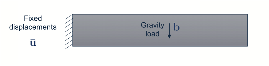
Figure 1: Cantilever beam considered in this example.

Strong Form

We consider the deformation of an elastic body undergoing finite strains. The balance of linear momentum in the reference configuration reads:

\[ \nabla \cdot \mathbf{P} + \mathbf{b} = 0 \quad \text{in } \mathbf{\Omega} \]

\[ \begin{cases} \mathbf{u} = \overline{\mathbf{u}} & \text{ on } \mathbf{\Gamma_u} \\ \mathbf{P} \cdot \mathbf{n} = \overline{\mathbf{t}} & \text{ on } \mathbf{\Gamma_t} \end{cases} \]

We consider the equilibrium problem in the domain \(\mathbf{\Omega}\), governed by the divergence operator acting on the First Piola–Kirchhoff stress tensor \(\mathbf{P}\) and the body forces \(\mathbf{b}\) per unit reference volume. The boundary \(\partial \mathbf{\Omega}\) is decomposed into \(\mathbf{\Gamma_u}\) and \(\mathbf{\Gamma_t}\), which are disjoint. On \(\mathbf{\Gamma_u}\), the displacement field \(\mathbf{u}\) is prescribed by \(\overline{\mathbf{u}}\), defining the Dirichlet (essential) boundary condition. On \(\mathbf{\Gamma_t}\), the traction vector \(\overline{\mathbf{t}}\) is applied through the action of the stress tensor \(\mathbf{P}\) on the outward unit normal vector \(\mathbf{n}\), defining the Neumann (natural) boundary condition. To account for large deformations, Hencky (logarithmic) strain measures are employed, allowing the constitutive response to follow the structure of Hooke’s law while incorporating geometric nonlinearities through the kinematics.

Constitutive model

To model large-strain elastic behavior, we begin with the deformation gradient

\[ \mathbf{F} = \frac{\partial \mathbf{x}}{\partial \mathbf{X}}, \]

which maps an infinitesimal material line element in the reference configuration to the current configuration. The deformation gradient contains both stretch and rigid-body rotation.

Using the polar decomposition theorem, the deformation gradient can be written as

\[ \mathbf{F} = \mathbf{R}\mathbf{U} = \mathbf{V}\mathbf{R}, \]

where

• \(\mathbf{R}\) is a proper orthogonal rotation tensor,
• \(\mathbf{U}\) is the right stretch tensor,
• \(\mathbf{V}\) is the left stretch tensor.

Since rigid-body rotations do not contribute to strain, they are removed by forming the right Cauchy–Green deformation tensor

\[ \mathbf{C} = \mathbf{F}^{\mathrm T}\mathbf{F}. \]

Substituting the polar decomposition gives

\[ \mathbf{C} = (\mathbf{R}\mathbf{U})^{\mathrm T} (\mathbf{R}\mathbf{U}) = \mathbf{U}^{\mathrm T} \mathbf{R}^{\mathrm T} \mathbf{R} \mathbf{U} = \mathbf{U}^{2}, \]

because \(\mathbf{R}^{\mathrm T}\mathbf{R}=\mathbf{I}\) and \(\mathbf{U}\) is symmetric. Consequently, the tensor \(\mathbf{C}\) contains only stretch information, while all rigid-body rotations are eliminated through the multiplication \(\mathbf{F}^{\mathrm T}\mathbf{F}\).

The Hencky (logarithmic) strain tensor is then defined as

\[ \mathbf{H} = \frac{1}{2}\ln(\mathbf{C}) = \ln(\mathbf{U}). \]

The logarithmic strain is particularly attractive for finite-deformation elasticity because it measures strain directly from the principal stretches and reduces to the infinitesimal strain tensor in the small-deformation limit.

The strain energy density \(\Psi\) is defined as a function of \(\mathbf{H}\). The Hencky stress \(\mathbf{T}\) is work-conjugate to \(\mathbf{H}\):

\[ \dot{\Psi} = \mathbf{P} : \dot{\mathbf{F}} = \mathbf{T} : \dot{\mathbf{H}} \]

The Hencky strain energy density function for isotropic materials is defined as

\begin{equation} \Psi(\mathbf{H}) = \mu\, \mathbf{H}:\mathbf{H} + \frac{\lambda}{2}\, \left(\mathrm{tr}(\mathbf{H})\right)^2, \label{eq:hencky_energy} \end{equation}

where \(\mu\) and \(\lambda\) are the Lamé parameters. The work-conjugate stress tensor is obtained by differentiating the strain energy density with respect to the Hencky strain:

\begin{equation} \mathbf{T} = \frac{\partial \Psi}{\partial \mathbf{H}} = 2\mu\,\mathbf{H} + \lambda\,\mathrm{tr}(\mathbf{H})\,\mathbf{I} = \mathbb{D}:\mathbf{H}, \end{equation}

The second Piola–Kirchhoff stress tensor \(\mathbf{S}\) follows from the chain rule:

\[ \mathbf{S} = 2 \frac{\partial \Psi}{\partial \mathbf{C}} = 2 \, \mathbf{T} : \frac{\partial \mathbf{H}}{\partial \mathbf{C}} \]

Finally, the first Piola–Kirchhoff stress tensor is:

\begin{equation} \mathbf{P} = \mathbf{F} \mathbf{S} \label{eq:piola} \end{equation}

Weak Form

The weak form of the nonlinear elastic problem is obtained by multiplying the balance equation by an admissible test function \(\delta \mathbf{u}\) and integrating over the reference configuration:

\[ \begin{array}{c} \int_{\mathbf{\Omega}} \nabla \delta \mathbf{u} : \mathbf{P}(\mathbf{u}) \, d\Omega - \int_{\mathbf{\Omega}} \delta \mathbf{u} \cdot \mathbf{b} \, d\Omega - \int_{\mathbf{\Gamma_t}} \delta \mathbf{u} \cdot \overline{\mathbf{t}} \, d\Gamma - \int_{\mathbf{\Gamma_u}} \delta \mathbf{u} \cdot \left( \mathbf{P} \cdot \mathbf{n} \right) \, d\Gamma = 0 , \, \, \, \forall \, \delta \mathbf{u} \in \mathbf{H}^1(\mathbf{\Omega}) \end{array} \]

We seek \(\mathbf{u} \in \mathbf{H}^1(\mathbf{\Omega})\) such that \(\mathbf{u} = 0\) on \(\mathbf{\Gamma_u}\), and satisfying the weak form.

\[ \begin{array}{c} \int_{\mathbf{\Omega}} \nabla \delta \mathbf{u} : \mathbf{P}(\mathbf{u}) \, d\Omega = \int_{\mathbf{\Omega}} \delta \mathbf{u} \cdot \mathbf{b} \, d\Omega + \int_{\mathbf{\Gamma_t}} \delta \mathbf{u} \cdot \overline{\mathbf{t}} \, d\Gamma , \, \, \, \forall \, \delta \mathbf{u} \in \mathbf{H}^1_0(\mathbf{\Omega}) \text{ with } \delta \mathbf{u} = \mathbf{0} \text{ on } \mathbf{\Gamma_u} \end{array} \]

Linearization

The nonlinear weak form is solved using a Newton–Raphson scheme. Linearization about the current iterate \(\mathbf{u}\) yields:

\[ \mathcal{R}(\mathbf{u}_0 + \Delta \mathbf{u}; \delta \mathbf{u}) \approx \mathcal{R}(\mathbf{u}_0; \delta \mathbf{u}) + D\mathcal{R}(\mathbf{u}_0)[\Delta \mathbf{u}; \delta \mathbf{u}] + \mathcal{O}(\|\Delta \mathbf{u}\|^2) \]

\[ \mathcal{R}(\mathbf{u}_0; \delta \mathbf{u}) = \int_{\Omega_0} \mathbf{P}(\mathbf{u}) : \nabla \delta \mathbf{u} \, dV - \int_{\Omega_0} \delta \mathbf{u} \cdot \mathbf{b} \, dV - \int_{\Gamma_t} \delta \mathbf{u} \cdot \bar{\mathbf{t}} \, dA. \]

\[ D\mathcal{R}(\mathbf{u}_0)[\Delta \mathbf{u}; \delta \mathbf{u}] =\int_{\Omega_0} \delta \mathbf{P}: \nabla \delta \mathbf{u} d V = \int_{\Omega_0}(\nabla \delta \mathbf{u}): \frac{\partial \mathbf{P}}{\partial \mathbf{F}}:(\nabla \Delta \mathbf{u}) d V \]

The final equation after linearization reads and assembled in the weak form is as follows, in the code is well know as lef hand side and right hand side respectively.

\[ \int_{\Omega_0}(\nabla \delta \mathbf{u}): \frac{\partial \mathbf{P}}{\partial \mathbf{F}}\left(\mathbf{u}^k\right):(\nabla \Delta \mathbf{u}) d V=-\left[\int_{\Omega_0} \mathbf{P}\left(\mathbf{u}^k\right): \nabla \delta \mathbf{u} d V-\int_{\Omega_0} \delta \mathbf{u} \cdot \mathbf{b} d V-\int_{\Gamma_t} \delta \mathbf{u} \cdot \mathbf{t}_0 d A\right] \quad, \, \, \, \forall \delta \mathbf{u} \in \mathbf{H}^1_0(\Omega) \]

The total derivative of \(\mathbf{P}\) or what is called the tangent stifness matrix can be computed using the chain rule:

\begin{equation} \delta \mathbf{P} = \delta \mathbf{F} \cdot \mathbf{T} : \left(2 \frac{\partial \mathbf{H}}{\partial \mathbf{C}}\right) + \mathbf{F} \cdot \delta \mathbf{T} : \left(2 \frac{\partial \mathbf{H}}{\partial \mathbf{C}}\right) + \mathbf{F} \cdot \mathbf{T} : \left(2 \frac{\partial^2 \mathbf{H}}{\partial \mathbf{C}^2} : \delta \mathbf{C}\right) \label{eq:dP} \end{equation}

So we can see in above equation that we need to find \(\delta \mathbf{C}\) and \(\delta \mathbf{T}\) by using the chain rule once more being careful that we are dealing with tensorial quantities.

The variation of \(\mathbf{C}\) becomes

\[ \delta \mathbf{C} = \mathbf{F}^\mathrm{T} (\delta \mathbf{F}) + (\delta \mathbf{F})^\mathrm{T} \mathbf{F} \]

which defines the partial derivative of \(\mathbf{C}\) with respect to \(\mathbf{F}\) as

\[ \frac{\partial \mathbf{C}}{\partial \mathbf{F}}=\mathbf{I} \otimes \mathbf{F}+\mathbf{F} \otimes \mathbf{I} \]

The variation of the Hencky stress, \(\mathbf{T}\) is found by exploiting the relationship between the Hencky strain and the right Cauchy-Green tensor, is then

\[ \delta \mathbf{T}=\frac{\partial \mathbf{T}}{\partial \mathbf{H}}: \delta \mathbf{H}=\frac{\partial \mathbf{T}}{\partial \mathbf{H}}:\left(2 \frac{\partial \mathbf{H}}{\partial \mathbf{C}}: \delta \mathbf{C}\right) . \]

\[ \delta \mathbf{T}=\frac{\partial \mathbf{T}}{\partial \mathbf{H}}: \delta \mathbf{H}=\frac{\partial \mathbf{T}}{\partial \mathbf{H}}:\left(2 \frac{\partial \mathbf{H}}{\partial \mathbf{C}}: \delta \mathbf{C}\right) \]

Replacing in equation \eqref{eq:dP}

\[ \delta \mathbf{P}=\delta \mathbf{F} \cdot \mathbf{T}: 2 \frac{\partial \mathbf{H}}{\partial \mathbf{C}}+\mathbf{F} \cdot \mathbf{T}:\left(2 \frac{\partial^2 \mathbf{H}}{\partial \mathbf{C}^2}: \delta \mathbf{C}\right) + \mathbf{F} \cdot\left[\mathbb{D}: \frac{\partial \mathbf{H}}{\partial \mathbf{C}}: \delta \mathbf{C}\right]: 2 \frac{\partial \mathbf{H}}{\partial \mathbf{C}} \]

\[ \delta \mathbf{P}=\delta \mathbf{F} \cdot \mathbf{T}: 2 \frac{\partial \mathbf{H}}{\partial \mathbf{C}}+\mathbf{F} \cdot\left[2 \frac{\partial^2 \mathbf{H}}{\partial \mathbf{C}^2}: \mathbf{T}+ \frac{1}{2}\frac{\partial \mathbf{H}}{\partial \mathbf{C}}: \mathbb{D}: \frac{\partial \mathbf{H}}{\partial \mathbf{C}}\right]: \delta \mathbf{C} \]

The resulting variation of \(\mathbf{P}\) can be expressed as comparing to the above equation:

\[ \delta \mathbf{P} = \frac{\partial \mathbf{P}}{\partial \mathbf{F}} : \delta \mathbf{F} \]

where the partial derivative is defined as :

\begin{equation} \frac{\partial \mathbf{P}}{\partial \mathbf{F}} = \mathbf{I} \otimes \mathbf{S} + \mathbf{F} : \left[\frac{1}{2}\left(4\frac{\partial^2 \mathbf{H}}{\partial \mathbf{C}^2} : \mathbf{T} + \frac{\partial \mathbf{H}}{\partial \mathbf{C}} : \mathbb{D} : \frac{\partial \mathbf{H}}{\partial \mathbf{C}}\right)\right] : \frac{\partial \mathbf{C}}{\partial \mathbf{F}} \label{eq:tangent} \end{equation}

Discretization

After discretization and linearization using the Newton–Raphson method, the nonlinear equilibrium equations are reduced at each iteration to a linear system of algebraic equations replacing with the respective shape function \(\mathbf{N}\). The right-hand side residual vector is expressed as \(\mathbf{R}\).

\[ \Delta \mathbf{u}^h = \sum_\beta \mathbf{N}_\beta \Delta \mathbf{d}_\beta, \quad \delta \mathbf{u}^h = \sum_\alpha \mathbf{N}_\alpha \delta \mathbf{d}_\alpha. \]

\[ \mathbf{K}_{\alpha \beta} = \int_{\Omega_0} (\nabla \mathbf{N}_\alpha) : \frac{\partial \mathbf{P}}{\partial \mathbf{F}} : (\nabla \mathbf{N}_\beta) \, dV \]

Implementation

This section outlines the main implementation aspects of the nonlinear elastic solver. The overall structure follows closely the workflow introduced in VEC-0: Linear elasticity, with extensions required to handle finite strains and nonlinear material response. The following steps are performed:

• definition of the spatial dimension and mesh entities,
• initialization of MoFEM, PETSc, and MOAB data structures,
• registration of the MoFEM discrete manager with PETSc,
• creation of the MOAB and MoFEM core objects,
• setup of logging channels for monitoring solver behavior.

The function Example::setupProblem() is identical to that used in VEC-0: Linear elasticity. The displacement field \(\mathbf{u}\) is approximated in an \(H^1\)-conforming space, using the AINSWORTH_LEGENDRE_BASE with polynomial order 2 by default. Boundary conditions are imposed using MoFEM operators, as illustrated below:

 
MoFEMErrorCode NonlinearElasticExample::boundaryCondition() {
  MoFEMFunctionBegin;
  auto *pipeline_mng = mField.getInterface<PipelineManager>();
  auto simple = mField.getInterface<Simple>();
  auto bc_mng = mField.getInterface<BcManager>();
  auto time_scale = boost::make_shared<ExampleTimeScale>();
 
  CHKERR BoundaryNaturalBC::AddFluxToPipeline<OpForce>::add(
      pipeline_mng->getOpBoundaryRhsPipeline(), mField, "U", {time_scale},
      "FORCE", "PRESSURE", Sev::inform);
 
  //! [Define gravity vector]
  CHKERR DomainNaturalBC::AddFluxToPipeline<OpBodyForce>::add(
      pipeline_mng->getOpDomainRhsPipeline(), mField, "U", {time_scale},
      "BODY_FORCE", Sev::inform);
 
  // Essential BC
  CHKERR bc_mng->removeBlockDOFsOnEntities(simple->getProblemName(), "REMOVE_X",
                                           "U", 0, 0);
  CHKERR bc_mng->removeBlockDOFsOnEntities(simple->getProblemName(), "REMOVE_Y",
                                           "U", 1, 1);
  CHKERR bc_mng->removeBlockDOFsOnEntities(simple->getProblemName(), "REMOVE_Z",
                                           "U", 2, 2);
  CHKERR bc_mng->pushMarkDOFsOnEntities<DisplacementCubitBcData>(
      simple->getProblemName(), "U");
 
  MoFEMFunctionReturn(0);
}

Operators are pushed to the pipeline using the same integration rules as in VEC-0: Linear elasticity. This ensures consistency between linear and nonlinear formulations.

Hencky stress

The Hencky stress template is used to calculate the equation \( \eqref{eq:hencky_stress} \) . This loop applies Hooke’s law to the logarithmic strain at each Gauss point, producing the Hencky stress that drives the nonlinear solve. Material block operations follow the same structure as in VEC-0: Linear elasticity, since the material response remains linear isotropic in terms of the chosen strain measure.

template <int DIM, typename DomainEleOp, int S>
struct OpCalculateHenckyStressImpl<DIM, GAUSS, DomainEleOp, S>
    : public DomainEleOp {
 
  OpCalculateHenckyStressImpl(const std::string field_name,
                              boost::shared_ptr<CommonData> common_data)
      : DomainEleOp(field_name, DomainEleOp::OPROW),
        commonDataPtr(common_data) {
    std::fill(&DomainEleOp::doEntities[MBEDGE],
              &DomainEleOp::doEntities[MBMAXTYPE], false);
  }
 
  MoFEMErrorCode doWork(int side, EntityType type, EntData &data) {
    MoFEMFunctionBegin;
 
    FTensor::Index<'i', DIM> i;
    FTensor::Index<'j', DIM> j;
    FTensor::Index<'k', DIM> k;
    FTensor::Index<'l', DIM> l;
 
    // const size_t nb_gauss_pts = matGradPtr->size2();
    const size_t nb_gauss_pts = DomainEleOp::getGaussPts().size2();
    auto t_D = getFTensor4DdgFromMat<DIM, DIM, S>(*commonDataPtr->matDPtr);
    auto t_logC = getFTensor2SymmetricFromMat<DIM>(commonDataPtr->matLogC);
    constexpr auto size_symm = (DIM * (DIM + 1)) / 2;
    commonDataPtr->matHenckyStress.resize(nb_gauss_pts, size_symm, false);
    auto t_T = getFTensor2SymmetricFromMat<DIM>(commonDataPtr->matHenckyStress);
 
    for (size_t gg = 0; gg != nb_gauss_pts; ++gg) {
      t_T(i, j) = t_D(i, j, k, l) * t_logC(k, l);
      ++t_logC;
      ++t_T;
      ++t_D;
    }
 
    MoFEMFunctionReturn(0);
  }
 
private:
  boost::shared_ptr<CommonData> commonDataPtr;
};
 

First Piola–Kirchhoff stress

The first Piola–Kirchhoff stress tensor from the equation \( \eqref{eq:piola} \) is obtained from the second Piola–Kirchhoff stress using the chain rule associated with the Hencky strain definition. This stress measure enters directly the weak form and residual evaluation

template <int DIM, typename DomainEleOp, int S>
struct OpCalculatePiolaStressImpl<DIM, GAUSS, DomainEleOp, S>
    : public DomainEleOp {
 
  OpCalculatePiolaStressImpl(const std::string field_name,
                             boost::shared_ptr<CommonData> common_data)
      : DomainEleOp(field_name, DomainEleOp::OPROW),
        commonDataPtr(common_data) {
    std::fill(&DomainEleOp::doEntities[MBEDGE],
              &DomainEleOp::doEntities[MBMAXTYPE], false);
  }
 
  MoFEMErrorCode doWork(int side, EntityType type, EntData &data) {
    MoFEMFunctionBegin;
 
    FTensor::Index<'i', DIM> i;
    FTensor::Index<'j', DIM> j;
    FTensor::Index<'k', DIM> k;
    FTensor::Index<'l', DIM> l;
 
    constexpr auto t_kd = FTensor::Kronecker_Delta<int>();
 
    // const size_t nb_gauss_pts = matGradPtr->size2();
    const size_t nb_gauss_pts = DomainEleOp::getGaussPts().size2();
#ifdef HENCKY_SMALL_STRAIN
    auto t_D = getFTensor4DdgFromMat<DIM, DIM, S>(*commonDataPtr->matDPtr);
#endif
    auto t_logC = getFTensor2SymmetricFromMat<DIM>(commonDataPtr->matLogC);
    auto t_logC_dC = getFTensor4DdgFromMat<DIM, DIM>(commonDataPtr->matLogCdC);
    constexpr auto size_symm = (DIM * (DIM + 1)) / 2;
    commonDataPtr->matFirstPiolaStress.resize(nb_gauss_pts, DIM * DIM, false);
    commonDataPtr->matSecondPiolaStress.resize(nb_gauss_pts, size_symm, false);
    auto t_P = getFTensor2FromMat<DIM, DIM>(commonDataPtr->matFirstPiolaStress);
    auto t_T = getFTensor2SymmetricFromMat<DIM>(commonDataPtr->matHenckyStress);
    auto t_S =
        getFTensor2SymmetricFromMat<DIM>(commonDataPtr->matSecondPiolaStress);
    auto t_grad = getFTensor2FromMat<DIM, DIM>(*(commonDataPtr->matGradPtr));
 
    for (size_t gg = 0; gg != nb_gauss_pts; ++gg) {
 
#ifdef HENCKY_SMALL_STRAIN
      t_P(i, j) = t_D(i, j, k, l) * t_grad(k, l);
#else
      FTensor::Tensor2<double, DIM, DIM> t_F;
      t_F(i, j) = t_grad(i, j) + t_kd(i, j);
      t_S(k, l) = t_T(i, j) * t_logC_dC(i, j, k, l);
      t_P(i, l) = t_F(i, k) * t_S(k, l);
#endif
 
      ++t_grad;
      ++t_logC;
      ++t_logC_dC;
      ++t_P;
      ++t_T;
      ++t_S;
#ifdef HENCKY_SMALL_STRAIN
      ++t_D;
#endif
    }
 
    MoFEMFunctionReturn(0);
  }
 
private:
  boost::shared_ptr<CommonData> commonDataPtr;
};

Pushing left hand side

The domain tangent stiffness matrix is assembled by pushing the corresponding left-hand side operators to the pipeline. The operator factory opFactoryDomainLhs is used for this purpose:

template <int DIM, AssemblyType A, IntegrationType I, typename DomainEleOp>
MoFEMErrorCode opFactoryDomainLhs(
    MoFEM::Interface &m_field,
    boost::ptr_deque<ForcesAndSourcesCore::UserDataOperator> &pip,
    std::string field_name, boost::shared_ptr<HenckyOps::CommonData> common_ptr,
    Sev sev) {
  MoFEMFunctionBegin;
 
  using B = typename FormsIntegrators<DomainEleOp>::template Assembly<
      A>::template BiLinearForm<I>;
  using OpKPiola = typename B::template OpGradTensorGrad<1, DIM, DIM, -1>;
 
  using H = HenckyIntegrators<DomainEleOp>;
  // Assumes constant D matrix per entity
  pip.push_back(new typename H::template OpHenckyTangent<DIM, I, 0>(
      field_name, common_ptr));
  pip.push_back(
      new OpKPiola(field_name, field_name, common_ptr->getMatTangent()));
 
  MoFEMFunctionReturn(0);
}
 
template <int DIM, AssemblyType A, IntegrationType I, typename DomainEleOp>
MoFEMErrorCode opFactoryDomainLhs(
    MoFEM::Interface &m_field,
    boost::ptr_deque<ForcesAndSourcesCore::UserDataOperator> &pip,
    std::string field_name, std::string block_name, Sev sev, double scale = 1) {
  MoFEMFunctionBegin;
 
  auto common_ptr = commonDataFactory<DIM, I, DomainEleOp>(
      m_field, pip, field_name, block_name, sev, scale);
  CHKERR opFactoryDomainLhs<DIM, A, I, DomainEleOp>(m_field, pip, field_name,
                                                    common_ptr, sev);
 
  MoFEMFunctionReturn(0);
}

Material tangent implementation

Here we assemble the material tangent matrix at each Gauss point. The nonlinearity is present from the outset through the full finite-strain kinematics, since the formulation is expressed in terms of the deformation gradient. The Hencky tangent operator defined in equation \eqref{eq:tangent}, which consistently accounts for geometric nonlinear effects, is therefore implemented within this complete finite-strain framework.

template <int DIM, typename DomainEleOp, int S>
struct OpHenckyTangentImpl<DIM, GAUSS, DomainEleOp, S> : public DomainEleOp {
  OpHenckyTangentImpl(const std::string field_name,
                      boost::shared_ptr<CommonData> common_data,
                      boost::shared_ptr<MatrixDouble> mat_D_ptr = nullptr)
      : DomainEleOp(field_name, DomainEleOp::OPROW),
        commonDataPtr(common_data) {
    std::fill(&DomainEleOp::doEntities[MBEDGE],
              &DomainEleOp::doEntities[MBMAXTYPE], false);
    if (mat_D_ptr)
      matDPtr = mat_D_ptr;
    else
      matDPtr = commonDataPtr->matDPtr;
  }
 
  MoFEMErrorCode doWork(int side, EntityType type, EntData &data) {
    MoFEMFunctionBegin;
 
    FTensor::Index<'i', DIM> i;
    FTensor::Index<'j', DIM> j;
    FTensor::Index<'k', DIM> k;
    FTensor::Index<'l', DIM> l;
    FTensor::Index<'m', DIM> m;
    FTensor::Index<'n', DIM> n;
    FTensor::Index<'o', DIM> o;
    FTensor::Index<'p', DIM> p;
 
    constexpr auto t_kd = FTensor::Kronecker_Delta<int>();
    // const size_t nb_gauss_pts = matGradPtr->size2();
    const size_t nb_gauss_pts = DomainEleOp::getGaussPts().size2();
    commonDataPtr->matTangent.resize(nb_gauss_pts, DIM * DIM * DIM * DIM);
    auto dP_dF =
        getFTensor4FromMat<DIM, DIM, DIM, DIM>(commonDataPtr->matTangent);
 
    auto t_D = getFTensor4DdgFromMat<DIM, DIM, S>(*matDPtr);
    auto t_eig_val = getFTensor1FromMat<DIM>(commonDataPtr->matEigVal);
    auto t_eig_vec = getFTensor2FromMat<DIM, DIM>(commonDataPtr->matEigVec);
    auto t_T = getFTensor2SymmetricFromMat<DIM>(commonDataPtr->matHenckyStress);
    auto t_S =
        getFTensor2SymmetricFromMat<DIM>(commonDataPtr->matSecondPiolaStress);
    auto t_grad = getFTensor2FromMat<DIM, DIM>(*(commonDataPtr->matGradPtr));
    auto t_logC_dC = getFTensor4DdgFromMat<DIM, DIM>(commonDataPtr->matLogCdC);
 
    for (size_t gg = 0; gg != nb_gauss_pts; ++gg) {
 
#ifdef HENCKY_SMALL_STRAIN
      dP_dF(i, j, k, l) = t_D(i, j, k, l);
#else
 
      FTensor::Tensor2<double, DIM, DIM> t_F;
      t_F(i, j) = t_grad(i, j) + t_kd(i, j);
 
      // rare case when two eigen values are equal
      auto nb_uniq = get_uniq_nb<DIM>(&t_eig_val(0));
      FTensor::Tensor4<double, DIM, DIM, DIM, DIM> dC_dF;
      dC_dF(i, j, k, l) = (t_kd(i, l) * t_F(k, j)) + (t_kd(j, l) * t_F(k, i));
 
      auto TL = EigenMatrix::getDiffDiffMat(t_eig_val, t_eig_vec, f, d_f, dd_f,
                                            t_T, nb_uniq);
      TL(i, j, k, l) *= 4;
      FTensor::Ddg<double, DIM, DIM> P_D_P_plus_TL;
      P_D_P_plus_TL(i, j, k, l) =
          TL(i, j, k, l) +
          (t_logC_dC(i, j, o, p) * t_D(o, p, m, n)) * t_logC_dC(m, n, k, l);
      P_D_P_plus_TL(i, j, k, l) *= 0.5;
      dP_dF(i, j, m, n) = t_kd(i, m) * (t_kd(k, n) * t_S(k, j));
      dP_dF(i, j, m, n) +=
          t_F(i, k) * (P_D_P_plus_TL(k, j, o, p) * dC_dF(o, p, m, n));
 
#endif
 
      ++dP_dF;
 
      ++t_grad;
      ++t_eig_val;
      ++t_eig_vec;
      ++t_logC_dC;
      ++t_S;
      ++t_T;
      ++t_D;
    }
 
    MoFEMFunctionReturn(0);
  }
 
private:
  boost::shared_ptr<CommonData> commonDataPtr;
  boost::shared_ptr<MatrixDouble> matDPtr;
};
 

Pushing right hand side

The internal force vector is assembled using the right-hand side operator factory opFactoryDomainRhs:

template <int DIM, AssemblyType A, IntegrationType I, typename DomainEleOp>
MoFEMErrorCode opFactoryDomainRhs(
    MoFEM::Interface &m_field,
    boost::ptr_deque<ForcesAndSourcesCore::UserDataOperator> &pip,
    std::string field_name, boost::shared_ptr<HenckyOps::CommonData> common_ptr,
    Sev sev) {
  MoFEMFunctionBegin;
 
  using B = typename FormsIntegrators<DomainEleOp>::template Assembly<
      A>::template LinearForm<I>;
  using OpInternalForcePiola =
      typename B::template OpGradTimesTensor<1, DIM, DIM>;
  pip.push_back(
      new OpInternalForcePiola("U", common_ptr->getMatFirstPiolaStress()));
 
  MoFEMFunctionReturn(0);
}
 
template <int DIM, AssemblyType A, IntegrationType I, typename DomainEleOp>
MoFEMErrorCode opFactoryDomainRhs(
    MoFEM::Interface &m_field,
    boost::ptr_deque<ForcesAndSourcesCore::UserDataOperator> &pip,
    std::string field_name, std::string block_name, Sev sev, double scale = 1) {
  MoFEMFunctionBegin;
 
  auto common_ptr = commonDataFactory<DIM, I, DomainEleOp>(
      m_field, pip, field_name, block_name, sev, scale);
  CHKERR opFactoryDomainRhs<DIM, A, I, DomainEleOp>(m_field, pip, field_name,
                                                    common_ptr, sev);
 
  MoFEMFunctionReturn(0);
}

The operator computing the contraction of stresses with displacement gradients is implemented in finite_elements.hpp.

Solver

The nonlinear system is solved using PETSc’s time-stepping interface (TS), which internally employs a Newton–Raphson (SNES) solver at each time step. The nonlinear solver and all associated tolerances are configured through the call to TSSetFromOptions(ts), which parses the parameters provided in param_file.petsc. In addition, during the postprocessing stage, we define and register the set of variables to be visualized in ParaView, ensuring that the relevant fields are available for analysis and interpretation of the computed solution.

MoFEMErrorCode NonlinearElasticExample::TsSolve() {
  MoFEMFunctionBegin;
  auto *simple = mField.getInterface<Simple>();
  auto *pipeline_mng = mField.getInterface<PipelineManager>();
 
  auto dm = simple->getDM();
  auto ts = pipeline_mng->createTSIM();
 
  auto add_extra_finite_elements_to_solver_pipelines = [&]() {
    MoFEMFunctionBegin;
 
    auto pre_proc_ptr = boost::make_shared<FEMethod>();
    auto post_proc_rhs_ptr = boost::make_shared<FEMethod>();
    auto post_proc_lhs_ptr = boost::make_shared<FEMethod>();
 
    auto time_scale = boost::make_shared<ExampleTimeScale>();
 
    auto get_bc_hook_rhs = [this, pre_proc_ptr, time_scale]() {
      MoFEMFunctionBeginHot;
      CHKERR EssentialPreProc<DisplacementCubitBcData>(mField, pre_proc_ptr,
                                                       {time_scale}, false)();
      MoFEMFunctionReturnHot(0);
    };
 
    pre_proc_ptr->preProcessHook = get_bc_hook_rhs;
 
    auto get_post_proc_hook_rhs = [this, post_proc_rhs_ptr]() {
      MoFEMFunctionBegin;
      CHKERR EssentialPreProcReaction<DisplacementCubitBcData>(
          mField, post_proc_rhs_ptr, nullptr, Sev::verbose)();
      CHKERR EssentialPostProcRhs<DisplacementCubitBcData>(
          mField, post_proc_rhs_ptr, 1.)();
      MoFEMFunctionReturn(0);
    };
    auto get_post_proc_hook_lhs = [this, post_proc_lhs_ptr]() {
      MoFEMFunctionBegin;
      CHKERR EssentialPostProcLhs<DisplacementCubitBcData>(
          mField, post_proc_lhs_ptr, 1.)();
      MoFEMFunctionReturn(0);
    };
    post_proc_rhs_ptr->postProcessHook = get_post_proc_hook_rhs;
    post_proc_lhs_ptr->postProcessHook = get_post_proc_hook_lhs;
 
    // This is low level pushing finite elements (pipelines) to solver
    auto ts_ctx_ptr = getDMTsCtx(simple->getDM());
    ts_ctx_ptr->getPreProcessIFunction().push_front(pre_proc_ptr);
    ts_ctx_ptr->getPreProcessIJacobian().push_front(pre_proc_ptr);
    ts_ctx_ptr->getPostProcessIFunction().push_back(post_proc_rhs_ptr);
    ts_ctx_ptr->getPostProcessIJacobian().push_back(post_proc_lhs_ptr);
    MoFEMFunctionReturn(0);
  };
 
  // Add extra finite elements to SNES solver pipelines to resolve essential
  // boundary conditions
  CHKERR add_extra_finite_elements_to_solver_pipelines();
 
  auto create_monitor_fe = [dm](auto &&post_proc_fe) {
    return boost::make_shared<Monitor>(dm.get(), post_proc_fe);
  };
 
  // Set monitor which postprocessing results and saves them to the hard drive
  boost::shared_ptr<FEMethod> null_fe;
  if (postProcDomainFe)
    CHKERR postProcDomainFe->setTagsToTransfer(
        std::vector<Tag>(listTagsToTransfer));
  if (postProcBdyFe)
    CHKERR postProcBdyFe->setTagsToTransfer(
        std::vector<Tag>(listTagsToTransfer));
  auto monitor_ptr =
      create_monitor_fe(std::make_pair(postProcDomainFe, postProcBdyFe));
  CHKERR DMMoFEMTSSetMonitor(dm, ts, simple->getDomainFEName(), null_fe,
                             null_fe, monitor_ptr);
 
  // Set time solver
  double ftime = 1;
  CHKERR TSSetMaxTime(ts, ftime);
  CHKERR TSSetExactFinalTime(ts, TS_EXACTFINALTIME_MATCHSTEP);
 
  auto B = createDMMatrix(dm);
  CHKERR TSSetI2Jacobian(ts, B, B, PETSC_NULLPTR, PETSC_NULLPTR);
  auto D = createDMVector(simple->getDM());
  CHKERR TSSetSolution(ts, D);
  CHKERR TSSetFromOptions(ts);
 
  CHKERR TSElasticPostStep::postStepInitialise(this);
  CHKERR TSSetPreStep(ts, TSElasticPostStep::preStepFun);
  CHKERR TSSetPostStep(ts, TSElasticPostStep::postStepFun);
  CHKERR TSSolve(ts, NULL);
  CHKERR TSElasticPostStep::postStepDestroy();
 
  CHKERR TSGetTime(ts, &ftime);
 
  PetscInt steps, snesfails, rejects, nonlinits, linits;
  CHKERR TSGetStepNumber(ts, &steps);
  CHKERR TSGetSNESFailures(ts, &snesfails);
  CHKERR TSGetStepRejections(ts, &rejects);
  CHKERR TSGetSNESIterations(ts, &nonlinits);
  CHKERR TSGetKSPIterations(ts, &linits);
  MOFEM_LOG_C("EXAMPLE", Sev::inform,
              "steps %d (%d rejected, %d SNES fails), ftime %g, nonlinits "
              "%d, linits %d",
              steps, rejects, snesfails, ftime, nonlinits, linits);
 
  MoFEMFunctionReturn(0);
}

All flags introduced to param_file.petsc are introduced in the TSSetFromOptions(ts) function.

Getting norms

Solver statistics, including residual norms, number of nonlinear iterations, and linear solver iterations, are retrieved for post-analysis:

MoFEMErrorCode NonlinearElasticExample::gettingNorms() {
  MoFEMFunctionBegin;
 
  auto simple = mField.getInterface<Simple>();
  auto dm = simple->getDM();
 
  auto T = createDMVector(simple->getDM());
  CHKERR DMoFEMMeshToLocalVector(simple->getDM(), T, INSERT_VALUES,
                                 SCATTER_FORWARD);
  double nrm2;
  CHKERR VecNorm(T, NORM_2, &nrm2);
  MOFEM_LOG("EXAMPLE", Sev::inform) << "Solution norm " << nrm2;
 
  auto post_proc_norm_fe = boost::make_shared<DomainEle>(mField);
 
  auto post_proc_norm_rule_hook = [](int, int, int p) -> int { return 2 * p; };
  post_proc_norm_fe->getRuleHook = post_proc_norm_rule_hook;
 
  CHKERR AddHOOps<SPACE_DIM, SPACE_DIM, SPACE_DIM>::add(
      post_proc_norm_fe->getOpPtrVector(), {H1}, "GEOMETRY");
 
  enum NORMS { U_NORM_L2 = 0, PIOLA_NORM, LAST_NORM };
  auto norms_vec =
      createVectorMPI(mField.get_comm(),
                      (mField.get_comm_rank() == 0) ? LAST_NORM : 0, LAST_NORM);
  CHKERR VecZeroEntries(norms_vec);
 
  auto u_ptr = boost::make_shared<MatrixDouble>();
  post_proc_norm_fe->getOpPtrVector().push_back(
      new OpCalculateVectorFieldValues<SPACE_DIM>("U", u_ptr));
 
  post_proc_norm_fe->getOpPtrVector().push_back(
      new OpCalcNormL2Tensor1<SPACE_DIM>(u_ptr, norms_vec, U_NORM_L2));
 
  if (useAdolcMaterial == PETSC_TRUE) {
#ifdef WITH_ADOL_C
    if (physicalEquationsPtr) {
      CHKERR MatOps::OpMaterialFactory<MatOps::ELASTICITY, modelType>::
          opPostProcFactory(mField, post_proc_norm_fe->getOpPtrVector(), "U",
                            physicalEquationsPtr);
      auto m_P = physicalEquationsPtr->matOpsDataPtr->getCommonDataPtr("P");
      post_proc_norm_fe->getOpPtrVector().push_back(
          new OpCalcNormL2Tensor2<MAT_DIM, MAT_DIM>(m_P, norms_vec,
                                                        PIOLA_NORM));
    }
#else
    SETERRQ(PETSC_COMM_WORLD, MOFEM_DATA_INCONSISTENCY,
            "ADOL-C support is not enabled. Please reconfigure with "
            "-DWITH_ADOL_C=ON and recompile to use AdolC material model.");
#endif
  } else {
    auto common_ptr = commonDataFactory<SPACE_DIM, GAUSS, DomainEleOp>(
        mField, post_proc_norm_fe->getOpPtrVector(), "U", "MAT_ELASTIC",
        Sev::inform);
    post_proc_norm_fe->getOpPtrVector().push_back(
        new OpCalcNormL2Tensor2<SPACE_DIM, SPACE_DIM>(
            common_ptr->getMatFirstPiolaStress(), norms_vec, PIOLA_NORM));
  }
 
  CHKERR DMoFEMLoopFiniteElements(dm, simple->getDomainFEName(),
                                  post_proc_norm_fe);
 
  CHKERR VecAssemblyBegin(norms_vec);
  CHKERR VecAssemblyEnd(norms_vec);
 
  MOFEM_LOG_CHANNEL("SELF"); // Clear channel from old tags
  if (mField.get_comm_rank() == 0) {
    const double *norms;
    CHKERR VecGetArrayRead(norms_vec, &norms);
    MOFEM_TAG_AND_LOG("SELF", Sev::inform, "example")
        << "norm_u: " << std::scientific << std::sqrt(norms[U_NORM_L2]);
    MOFEM_TAG_AND_LOG("SELF", Sev::inform, "example")
        << "norm_piola: " << std::scientific << std::sqrt(norms[PIOLA_NORM]);
    CHKERR VecRestoreArrayRead(norms_vec, &norms);
  }
 
  MoFEMFunctionReturn(0);
}

Checking results

Basic verification checks are performed to ensure solver consistency and detect possible convergence issues:

MoFEMErrorCode NonlinearElasticExample::checkResults() {
  MoFEMFunctionBegin;
  PetscInt test_nb = 0;
  PetscBool test_flg = PETSC_FALSE;
  CHKERR PetscOptionsGetInt(PETSC_NULLPTR, "", "-test", &test_nb, &test_flg);
 
  if (test_flg) {
    if (test_nb >= 100) {
      CHKERR checkPiolaStress(test_nb);
      MoFEMFunctionReturnHot(0);
    }
 
    auto simple = mField.getInterface<Simple>();
    auto T = createDMVector(simple->getDM());
    CHKERR DMoFEMMeshToLocalVector(simple->getDM(), T, INSERT_VALUES,
                                   SCATTER_FORWARD);
    double nrm2;
    CHKERR VecNorm(T, NORM_2, &nrm2);
    MOFEM_LOG("EXAMPLE", Sev::verbose) << "Regression norm " << nrm2;
 
    double regression_value = 0;
    switch (test_nb) {
    case 1:
      regression_value = 3.5112e-01;
      break;
    case 2:
      regression_value = 1.8841e+00;
      break;
    case 3:
      regression_value = 1.8841e+00;
      break;
    default:
      SETERRQ(PETSC_COMM_WORLD, MOFEM_ATOM_TEST_INVALID, "Wrong test number.");
      break;
    }
    if (fabs(nrm2 - regression_value) > 1e-2)
      SETERRQ(PETSC_COMM_WORLD, MOFEM_ATOM_TEST_INVALID,
              "Regression test field; wrong norm value. %6.4e != %6.4e", nrm2,
              regression_value);
  }
  MoFEMFunctionReturn(0);
}

Running code and visualisation

Before running the simulation, verify the parameters in param_file.petsc. Only solver options relevant to the chosen linear solver should be enabled. For example:

## Linear solver
-ksp_type fgmres
-pc_type lu
-pc_factor_mat_solver_type mumps
-ksp_monitor

To run the three-dimensional case:

./nonlinear_elastic -file_name beam_3D.cub -order 2

For the two-dimensional case:

./nonlinear_elastic_2d -file_name beam_2D.cub -order 2

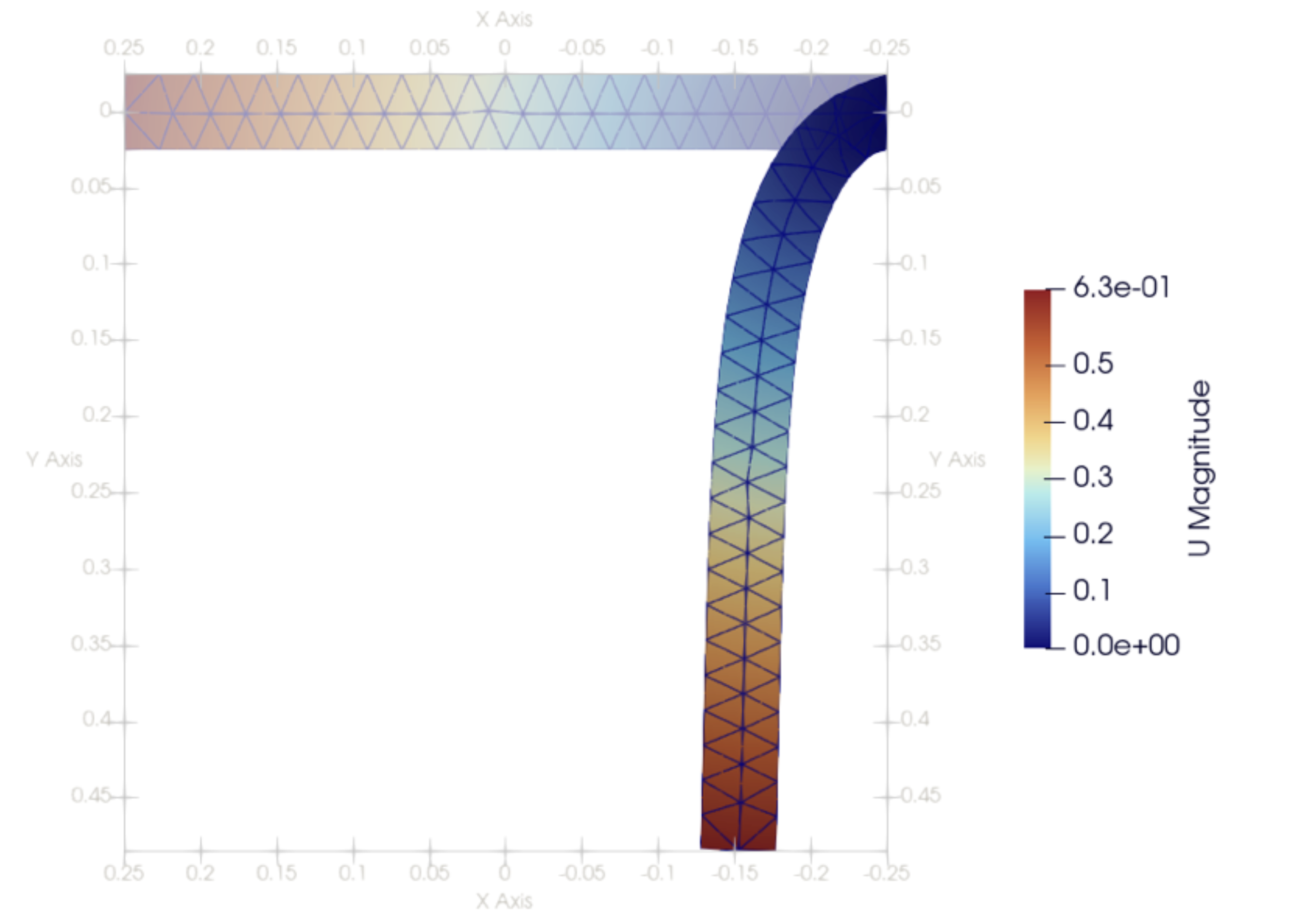
Figure 3: Deformation of cantilever beams in 2D. The color map represents the displacement magnitude.

With -snes_atol = 1e-8 and -snes_rtol = 1e-8, the convergence behavior shown in Figure 4 is obtained.

Source Files

The full source code associated with this tutorial is provided in:

• NonlinearElasticExample.hpp
• HenckyOps.hpp
• nonlinear_elastic.cpp