- Note
- Prerequisite of this tutorial is SCL-1: Poisson's equation (homogeneous BC)
- Note
- Intended learning outcome:
- idea of Boundary element in MoFEM and how to use it
- handling of non-homogeneous boundary conditions using least square approximation in MoFEM
- process of implementing additional User Data Operators (UDOs) to calculate and assemble non-homogeneous boundary condition
- practising on how to push the developed UDOs to the Pipeline
Introduction
The focus of our current tutorial is on solving Laplace-type partial differential equations (PDEs) Poisson Problem with non-homogenous Dirichlet boundary conditions. While the SCL-2: Poisson's equation (non-homogeneous BC) has designed for solving Dirichlet problems with homogeneous boundary conditions, this tutorial guides the methods to extend this to non-homogeneous cases and plot the solution.
We are also aiming to present MoFEM approaches for handling Dirichlet problems in addition to the least square approximation while establishing your necessary foundation in MoFEM as well. Prior to that, we would like to suggest understanding the operators(i.e. OpDomainLhsMatrixK and OpDomainRhsVectorF) in SCL-1: Poisson's equation (homogeneous BC) before proceeding to this tutorial.
Problem Statement
We are demonstrating an approach to solve a simple Poisson's problem with nonhomogenous BC and help you grasp the approach better. For this problem, we denote the domain as Ω, and Γ represents the Dirichlet boundary, as illustrated in Figure 1.
Thus, we are solving a sample problem with nonhomogeneous BCs to find \(\mathbf{u}\). such that:
Domain Equation:
\[ \begin{align} -\nabla \cdot\nabla u = f(\mathbf{x}) \,\,\, in \,\,\, \Omega \end{align} \]
Boundary condition:
\[ \begin{align} u = g(\mathbf{x}) \,\,\, on \,\,\,\Gamma \end{align} \]
Where f is the source term of the body and g is denoted as boundary function. However, if g is a constant everywhere (i.e. 0), we speak of homogeneous boundary conditions but in this problem, we are considering a spatially varying function \(g(\mathbf{x})\).
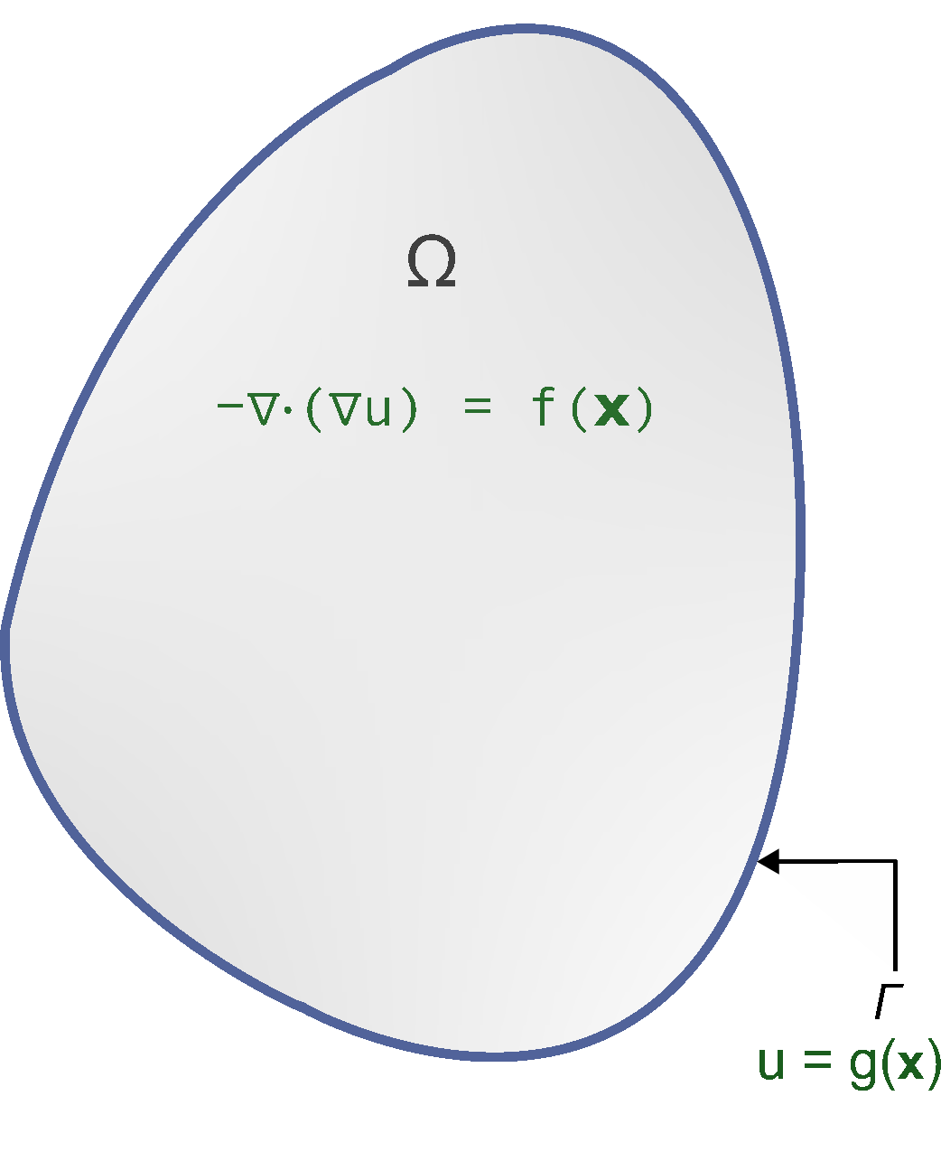
Figure 1: Nonhomogeneous problem Statement.
Numerical Scheme
In the context of solving this partial differential equation (PDE), Galerkin finite element methods with least square approximation have been executed to enforce nonhomogeneous boundary condition. We are also utilizing MoFEM libraries conforming finite element spaces with Least-Square approximation(LSA) for the boundary by minimizing the squared differences between the approximated values and the actual, similar to the following:
\[ \frac{1}{2}\int_{\Gamma} (u - g(\mathbf{x}))^2 \,d\Gamma \]
Remember, previously we derived a weak form for homogeneous BC in SCL-1: Poisson's equation (homogeneous BC). Following that approch, we can write similar weak form for our current problem for domain (Ω) and boundary(Γ) which also exists for \( \forall \,\delta u \) as follows:
\[ \begin{align} \int_{\Omega} \nabla \delta u \cdot \nabla u \,d\Omega = \int_{\Omega} \delta u \,f(\mathbf{x})\,d\Omega \quad\text{and} \end{align} \]
\[ \begin{align} \int_{\Gamma} \delta u \, \,d\Gamma = \int_{\Gamma} \delta u \,g(\mathbf{x})\,d\Gamma \end{align} \]
Approximation
In the context of finite element method, the problem will be solved numerically by approximating the scalar space \( \mathbf{H^1} \) by the discrete counterparts associated with our FE mesh of the computational domain \(\Omega\). To do that, we are utilizing two key components to solve: (i) \(N_{\alpha} \) and \(N_{\beta} \) are the shape functions for the field variable and for test functions respectively, (ii) \(\bar{u}_{\alpha}\) and \(\delta\bar{u}_{\beta}\) represent for 'n' number of DoF within that element to obtain the solution 'u' as stated below:
\[ \begin{align} u &= \sum_{\alpha=0}^{n-1} \mathbf{N}_{\alpha} \bar{u}_\alpha \,\,\text{and,}\\ {\delta u} &= \sum_{\beta=0}^{n-1}\mathbf{{N}_{\beta}} \delta\bar{u}_{\beta} \end{align} \]
Further, to assemble the element stiffness matrix we are indicating \(\alpha\) for the collums and \(\beta\) for rows. A typical approximation can be understood well in tutorial FUN-2: Hierarchical approximation. So, to approximate the fields based on the weak forms in equation (5) and (6) can be written as follows:
\[ \begin{equation} \sum_{\alpha=0}^{n-1} \sum_{\beta=0}^{n-1} \delta\bar{u}_{\beta} \left[\int_{\Omega} \nabla \mathbf{N}_{\alpha} \cdot \nabla \mathbf{N}_{\beta} \,d\Omega\right] \bar{u}_{\alpha} \,\,= \,\, \sum_{\beta=0}^{n-1} \delta \bar{u}_{\beta} \left[\int_{\Omega} f(\mathbf{x})\,\, \mathbf{N}_{\beta} \,d\Omega\right] \quad ;\,\forall \,\delta \bar{u}_{\beta} \end{equation} \]
and
\[ \begin{equation} \sum_{\alpha=0}^{n-1} \sum_{\beta=0}^{n-1} \delta\bar{u}_{\beta} \left[\int_{\Gamma} \mathbf{N}_{\alpha} \,\,\mathbf{N}_{\beta} \,d\Gamma\right] \bar{u}_{\alpha} \,\,= \,\,\sum_{\beta=0}^{n-1} \delta \bar{u}_{\beta} \left[\int_{\Gamma} g(\mathbf{x})\,\, \mathbf{N}_{\beta} \,d\Gamma\right]\quad ;\forall \,\delta \bar{u}_{\beta} \end{equation} \]
For a better understanding the implementation of the aboves in MoFEM, we are explaining the forms in two parts: domain and boundary. Also, let's say, we are naming the individuals for respective UDOs as follows,
\[ \mathbf{A_k} = \int_{\Omega} \nabla \mathbf{N}_{\alpha} \cdot \nabla \mathbf{N}_{\beta} \,d\Omega, \quad \mathbf{B_f} = \int_{\Omega} f(\mathbf{x})\,\,\mathbf{N}_{\beta} \,d\Omega\,\,\ \text{ |\,For Domain}, \]
and
\[ \mathbf{C_k} = \int_{\Gamma} \mathbf{N}_{\alpha} \cdot \mathbf{N}_{\beta} \,d\Gamma, \quad \mathbf{D_f} = \int_{\Gamma} g(\mathbf{x})\,\, \mathbf{N}_{\beta} \,d\Gamma \,\,\text{ |\,For Boundary}. \]
Additionally, a similar discretization and implementation approach was referred in tutorial SCL-1: Poisson's equation (homogeneous BC).
Problem formulation
Based on the above schemes, we are considering 4 operators in MoFEM. Let's say, we are naming those as follows:
Table 1: Operators for Domain and Boundary for Relevant Expresions
| Respective Operators |
| \(\mathbf{A_k} \text{is implemented in } \text{OpDomainLhs}\) |
| \(\mathbf{B_f} \text{is implemented in } \text{OpDomainRhs}\) |
| \(\mathbf{C_k} \text{is implemented in } \text{OpBoundaryLhs}\) |
| \(\mathbf{D_f} \text{is implemented in } \text{OpBoundaryRhs}\) |
The numerical scheme has several similarities with SCL-1: Poisson's equation (homogeneous BC) in terms of coding in MOFEM. Therefore, we are mostly going to discuss the critical parts of it in the next section comparing with the SCL-1: Poisson's equation (homogeneous BC).
Code Structure
Before we explore the implementation details of the User-Defined Operators (UDOs) in "poisson_2d_nonhomogeneous.hpp", let's take a look at the initial lines of code in the file. It includes MoFEM libraries inclusions for finite element functionality and alias definitions for declaration and initialization as follows:
#ifndef __POISSON2DNONHOMOGENEOUS_HPP__
#define __POISSON2DNONHOMOGENEOUS_HPP__
#include <stdlib.h>
typedef boost::function<
double(
const double,
const double,
const double)>
User Defined Operators(UDO)
MoFEM has an in-built extensive library consisting of operators and to implement those operators users need to create some new UDOs according to the problems and PDEs. First, let's look at the structure of a UDO so that users can also learn the general structure of any UDOs implemented in MoFEM.
OpDomainLhs()
For example, we can notice that our OpDomainLhs is similar to the OpDomainLhsMatrixK UDO in SCL-1: Poisson's equation (homogeneous BC). So, let's identify the differences bellow and then the further will be discussed:
public:
OpDomainLhs(std::string row_field_name, std::string col_field_name)
sYmm = true;
}
EntityType col_type,
EntData &row_data,
const int nb_row_dofs = row_data.
getIndices().size();
const int nb_col_dofs = col_data.
getIndices().size();
if (nb_row_dofs && nb_col_dofs) {
locLhs.resize(nb_row_dofs, nb_col_dofs, false);
locLhs.clear();
const int nb_integration_points =
getGaussPts().size2();
for (int gg = 0; gg != nb_integration_points; gg++) {
const double a = t_w * area;
for (int rr = 0; rr != nb_row_dofs; ++rr) {
for (int cc = 0; cc != nb_col_dofs; cc++) {
locLhs(rr, cc) += t_row_diff_base(
i) * t_col_diff_base(
i) *
a;
++t_col_diff_base;
}
++t_row_diff_base;
}
++t_w;
}
CHKERR MatSetValues<MoFEM::EssentialBcStorage>(
getKSPB(), row_data, col_data, &locLhs(0, 0), ADD_VALUES);
if (row_side != col_side || row_type != col_type) {
transLocLhs.resize(nb_col_dofs, nb_row_dofs, false);
noalias(transLocLhs) = trans(locLhs);
CHKERR MatSetValues<MoFEM::EssentialBcStorage>(
getKSPB(), col_data, row_data, &transLocLhs(0, 0), ADD_VALUES);
}
}
}
private:
boost::shared_ptr<std::vector<unsigned char>> boundaryMarker;
};
In the above, the class OpDomainLhs is inherited from OpFaceEle, which stands for the alias for the base class MoFEM::FaceElementForcesAndSourcesCore::UserDataOperator. Within this class, there are two public functions: OpDomainLhs() and doWork(). Here, the doWork() does the same as iNtegrate as in SCL-1: Poisson's equation (homogeneous BC). However, the difference is that we are using a different Lambda function to calculate the body source term. Alongside, we have got two private members named locLhs and transLocLhs. This follows the concept of data encapsulation to hide values and objects inside the class as much as possible.
locLhs
This private member object of type MatrixDouble is used to store the results of the calculation of the components of element stiffness matrix. Besides, this object is made private so that only member of the class has access to use this private object avoiding unpredictable consequences, i.e. errors.transLocLhs
This private member object also of type MatrixDouble is used to assemble the transpose of locLhs. This object is used only in function doWork() so it is also declared as a private object of the class OpDomainLhs.CHKERR MatSetValues
The code part is as follows: CHKERR MatSetValues<MoFEM::EssentialBcStorage>(
getKSPB(), row_data, col_data, &locLhs(0, 0), ADD_VALUES);
if (row_side != col_side || row_type != col_type) {
transLocLhs.resize(nb_col_dofs, nb_row_dofs, false);
noalias(transLocLhs) = trans(locLhs);
CHKERR MatSetValues<MoFEM::EssentialBcStorage>(
getKSPB(), col_data, row_data, &transLocLhs(0, 0), ADD_VALUES);
OpDomainRhs()
The characterization of OpDomainRhs is straightforward and also aligns with OpDomainRhsVectorF in the context of SCL-1 for solving Poisson's equation with homogeneous BC. However, there is a slight difference in the body source term. The accompanying code snippet illustrates in the following:
public:
sourceTermFunc(source_term_function) {}
if (nb_dofs) {
locRhs.resize(nb_dofs, false);
locRhs.clear();
const int nb_integration_points =
getGaussPts().size2();
for (int gg = 0; gg != nb_integration_points; gg++) {
const double a = t_w * area;
double body_source =
sourceTermFunc(t_coords(0), t_coords(1), t_coords(2));
for (int rr = 0; rr != nb_dofs; rr++) {
locRhs[rr] += t_base * body_source *
a;
++t_base;
}
++t_w;
++t_coords;
}
CHKERR VecSetValues<MoFEM::EssentialBcStorage>(
getKSPf(), data, &*locRhs.begin(), ADD_VALUES);
}
}
private:
};
In the above snippet, we can find a different body_source term which is calculated by calling a Lambda function sourceTermFunc() with coordinate(x, y, z) i.e. t_coords(0), t_coords(1), and t_coords(2) as arguments as follows:
double body_source =
sourceTermFunc(t_coords(0), t_coords(1), t_coords(2));
for (int rr = 0; rr != nb_dofs; rr++) {
locRhs[rr] += t_base * body_source *
a;
++t_base;
}
OpBoundaryLhs()
OpBoundaryLhs is focusing on the boundary( \( \Gamma\)) instead of the domain. So we're using OpEdgeEle instead of OpFaceEle. You can realize the fact easily that for 2D problems any boundary element type should be edge(1D) and for 3D problems it will be face(2D) type element.This operator is quite similar to our first operator, OpDomainLhs. Therefore we are not describing it again. Further, the code snippet is here:
public:
OpBoundaryLhs(std::string row_field_name, std::string col_field_name)
sYmm = true;
}
EntityType col_type,
EntData &row_data,
const int nb_row_dofs = row_data.
getIndices().size();
const int nb_col_dofs = col_data.
getIndices().size();
if (nb_row_dofs && nb_col_dofs) {
locBoundaryLhs.resize(nb_row_dofs, nb_col_dofs, false);
locBoundaryLhs.clear();
const int nb_integration_points =
getGaussPts().size2();
for (int gg = 0; gg != nb_integration_points; gg++) {
const double a = t_w * edge;
for (int rr = 0; rr != nb_row_dofs; ++rr) {
for (int cc = 0; cc != nb_col_dofs; cc++) {
locBoundaryLhs(rr, cc) += t_row_base * t_col_base *
a;
++t_col_base;
}
++t_row_base;
}
++t_w;
}
CHKERR MatSetValues<MoFEM::EssentialBcStorage>(
getKSPB(), row_data, col_data, &locBoundaryLhs(0, 0), ADD_VALUES);
if (row_side != col_side || row_type != col_type) {
transLocBoundaryLhs.resize(nb_col_dofs, nb_row_dofs, false);
noalias(transLocBoundaryLhs) = trans(locBoundaryLhs);
CHKERR MatSetValues<MoFEM::EssentialBcStorage>(
getKSPB(), col_data, row_data, &transLocBoundaryLhs(0, 0),
ADD_VALUES);
}
}
}
private:
};
OpBoundaryRhs()
If we compare the OpBoundaryRhs operator, it also closely resembles the OpDomainRhsVectorF operator in its structure. Additionally, it is also similar to OpBoundaryRhs. However, we are now using boundary_term here instead of body_source as follows:
double boundary_term =
boundaryFunc(t_coords(0), t_coords(1), t_coords(2));
for (int rr = 0; rr != nb_dofs; rr++) {
locBoundaryRhs[rr] += t_base * boundary_term *
a;
++t_base;
}
Main program (*.cpp)
This main class Poisson2DNonhomogeneous contains functions each of which is responsible for a certain task as described in SCL-1. However, in this case, we need to declare two functions as a global variable of sourceTermFunction and boundaryFunction. These functions are applicable for the operators OpDomainRhs and OpBoundaryRhs respectively. In addition to that, we have declared a vector type shared pointer 'boundaryMarker'. We will use and discuss while applying the boundary condition. The code snippet is as follows:
public:
private:
const double z) {
return 200 * sin(x * 10.) * cos(y * 10.);
}
const double z) {
return sin(x * 10.) * cos(y * 10.);
}
};
readMesh()
Next, this code defines function in MoFEM to loads and reads your mesh file.
setupProblem()
Since we are considering both domain and boundary, we need to add the domain and boundary field in the simpleInterface to setup the problem. Besides, we have selected the polynomial base function as AINSWORTH_BERNSTEIN_BEZIER_BASE and \( \mathbf{H^1}\) scalar space, where we are considering single(1) degree of freedom for each shape function has
boundaryCondition()
Next, we are proceeding to discuss the detail for setting up boundary condition. This code involves marking degrees of freedom on boundary entities, merging markers, and obtaining entities for field splitting in the following:
true);
boundaryMarker = bc_mng->getMergedBlocksMarker({
"BOUNDARY_CONDITION"});
bc_mng->getMergedBlocksRange({"BOUNDARY_CONDITION"});
}
The line bc_mng->pushMarkDOFsOnEntities(...) is used to collect the degrees of freedom (DOFs) of the entities only for marked block set ("BOUNDARY_CONDITION"). Then, the block sets are accumulated as in container and assembled in boundaryMarker. In addition, the `boundaryEntitiesForFieldsplit is to get the range/IDs for the blocks including vertex, edges or faces. It has been done to indicate the difference between the domain and boundary entities.
assembleSystem()
At this stage, we are all set to focus on assembling all we did before to the pipeline. However, we find some changes that happens here in codes compared with SCL-2: Poisson's equation (non-homogeneous BC). Before going to that, first we add operators to the OpDomainLhsPipeline using the AddHOOps function considering scalar space H1. Then we need to assemble to the pipeline for the domain using OpSetBc. Then push the main OpDomainLhs operator, and finally unset the assembly using OpUnSetBc. We will discuss it in detail after going through the code snippet in the following:
{
pipeline_mng->getOpDomainLhsPipeline(), {H1});
pipeline_mng->getOpDomainLhsPipeline().push_back(
pipeline_mng->getOpDomainLhsPipeline().push_back(
pipeline_mng->getOpDomainLhsPipeline().push_back(
}
{
pipeline_mng->getOpDomainRhsPipeline().push_back(
pipeline_mng->getOpDomainRhsPipeline().push_back(
pipeline_mng->getOpDomainRhsPipeline().push_back(
}
{
pipeline_mng->getOpBoundaryLhsPipeline().push_back(
pipeline_mng->getOpBoundaryLhsPipeline().push_back(
pipeline_mng->getOpBoundaryLhsPipeline().push_back(
}
{
pipeline_mng->getOpBoundaryRhsPipeline().push_back(
pipeline_mng->getOpBoundaryRhsPipeline().push_back(
pipeline_mng->getOpBoundaryRhsPipeline().push_back(
}
}
Here, the process involves using the OpSetBc, OpUnSetBc, and UDOs to push back to the RHS and LHS pipelines for assembling. Specifically, these operations are being carried out on the pipeline for the Domain and boundary in same way i.e. getOpDomainLhsPipeline(), OpBoundaryLhsPipeline. So we are only describing for only one set of assemble processes in the following:
The OpSetBc() object is responsible for assembling only for the boundary entities or everything except the boundary. In other words, when it is flagged 'true' it focuses exclusively on the domain entities and does not account for boundary entities tagged with the 'boundaryMarker.
{
pipeline_mng->getOpDomainLhsPipeline(), {H1});
pipeline_mng->getOpDomainLhsPipeline().push_back(
pipeline_mng->getOpDomainLhsPipeline().push_back(
pipeline_mng->getOpDomainLhsPipeline().push_back(
}
For example, when we assemble for the boundary, first we use OpSetBc(), then add OpBoundaryLhs and OpUnSetBc to the getOpBoundaryLhsPipeline() and getOpBoundaryLhsPipeline. To be noted that it's important to set the flag as false here.
To recapitulate, when we are assembling for the domain, OpSetBc() works for skipping(marked'true' to skip boundary) the boundary entities. On the other hand, it considers only the boundaries (marked 'false' to consider) when assembling only for boundary. And then push the UDO. Then OpUnSetBc() is used to set the index to the entities as it was initially.
setIntegrationRules()
Afterwards, the computation of LHS and RHS is defined in the setIntegrationRules. The instructions for the functions setIntegrationRules() is same as it was in SCL-1: Poisson's equation (homogeneous BC).
auto domain_rule_lhs = [](
int,
int,
int p) ->
int {
return 2 * (p - 1); };
auto domain_rule_rhs = [](
int,
int,
int p) ->
int {
return 2 * (p - 1); };
CHKERR pipeline_mng->setDomainLhsIntegrationRule(domain_rule_lhs);
CHKERR pipeline_mng->setDomainRhsIntegrationRule(domain_rule_rhs);
auto boundary_rule_lhs = [](
int,
int,
int p) ->
int {
return 2 * p; };
auto boundary_rule_rhs = [](
int,
int,
int p) ->
int {
return 2 * p; };
CHKERR pipeline_mng->setBoundaryLhsIntegrationRule(boundary_rule_lhs);
CHKERR pipeline_mng->setBoundaryLhsIntegrationRule(boundary_rule_rhs);
}
solveSystem()
To solve the problem, we remember that we made our assembling systems ready using the set/unseting process in boundaryCondition() for domain and boundaries as shown in Figure: 2 where we can consider the subscripts 'D' is for domain and 'B' for boundary.
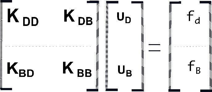
Figure 2: Solving approach
At this stage, we are not solving the system of equations directly using KSP solver as we did in SCL-1: Poisson's equation (homogeneous BC). Instead of that, we are proceeding to deploy a preconditioner to the solver named FIELDSPLIT. It splits the fields for domain and boundary as an option - yes/no if needed. The part of the code is as follows:
if (1) {
PC pc;
CHKERR KSPGetPC(ksp_solver, &pc);
PetscBool is_pcfs = PETSC_FALSE;
PetscObjectTypeCompare((PetscObject)pc, PCFIELDSPLIT, &is_pcfs);
if (is_pcfs == PETSC_TRUE) {
IS is_domain, is_boundary;
&boundaryEntitiesForFieldsplit);
CHKERR PCFieldSplitSetIS(pc, NULL, is_boundary);
CHKERR ISDestroy(&is_boundary);
}
}
The algorithm for the above code is to check whether the indices in the field were marked for domain or boundary. It set up the field-split solver using PETSc libraries for boundary entities(boundaryEntitiesForFieldsplit) and the remaining will be for the domain. During the iteration process, IS considers solving the option for domain and boundary so that the index sets are then used to configure the PCFIELDSPLIT solver to solve the appropriate blockset. Finally, the code releases the memory associated with the boundary index set and goes for KSP to solve. And to accumulate all these we followed by VecGhostUpdateBegin(), VecGhostUpdateEnd() and DMoFEMMeshToLocalVector to make things ready before getting the results.
CHKERR VecGhostUpdateBegin(
D, INSERT_VALUES, SCATTER_FORWARD);
CHKERR VecGhostUpdateEnd(
D, INSERT_VALUES, SCATTER_FORWARD);
}
The rest of the code including outputResults() and main function does the same as SCL-2: Poisson's equation (non-homogeneous BC)
Then, run the analysis and get the newly created output file, namely out_result.h5m. Convert it to *.vtk format. Then open it in Paraview and use the filter WarpByScalar, you will be able to see the deformation as bellow:
Results
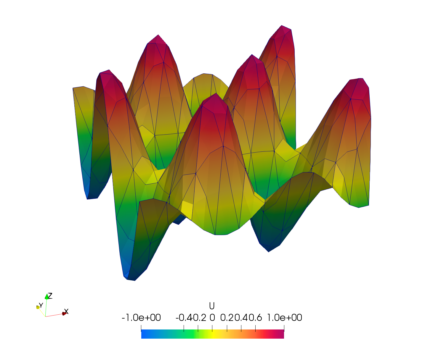
Figure 3: Poisson nonhomogeneous visualisation. Source term: 200sin(10x)cos(10y), boundary function: sin(10x)cos(10y)
Further requisite: https://en.wikiversity.org/wiki/Partial_differential_equations/Poisson_Equation.
Plain program
The plain program for both the implementation of the UDOs (*.hpp) and the main program (*.cpp) are as follows
Implementation of User Data Operators (*.hpp)
#ifndef __POISSON2DNONHOMOGENEOUS_HPP__
#define __POISSON2DNONHOMOGENEOUS_HPP__
typedef boost::function<
double(
const double,
const double,
const double)>
public:
OpDomainLhs(std::string row_field_name, std::string col_field_name)
sYmm = true;
}
MoFEMErrorCode doWork(
int row_side,
int col_side, EntityType row_type,
EntityType col_type,
EntData &row_data,
const int nb_row_dofs = row_data.
getIndices().size();
const int nb_col_dofs = col_data.
getIndices().size();
if (nb_row_dofs && nb_col_dofs) {
locLhs.resize(nb_row_dofs, nb_col_dofs, false);
locLhs.clear();
const double area = getMeasure();
const int nb_integration_points = getGaussPts().size2();
auto t_w = getFTensor0IntegrationWeight();
for (int gg = 0; gg != nb_integration_points; gg++) {
const double a = t_w * area;
for (int rr = 0; rr != nb_row_dofs; ++rr) {
for (int cc = 0; cc != nb_col_dofs; cc++) {
locLhs(rr, cc) += t_row_diff_base(
i) * t_col_diff_base(
i) *
a;
++t_col_diff_base;
}
++t_row_diff_base;
}
++t_w;
}
CHKERR MatSetValues<MoFEM::EssentialBcStorage>(
getKSPB(), row_data, col_data, &locLhs(0, 0), ADD_VALUES);
if (row_side != col_side || row_type != col_type) {
transLocLhs.resize(nb_col_dofs, nb_row_dofs, false);
noalias(transLocLhs) = trans(locLhs);
CHKERR MatSetValues<MoFEM::EssentialBcStorage>(
getKSPB(), col_data, row_data, &transLocLhs(0, 0), ADD_VALUES);
}
}
}
private:
boost::shared_ptr<std::vector<unsigned char>> boundaryMarker;
};
public:
sourceTermFunc(source_term_function) {}
if (nb_dofs) {
locRhs.resize(nb_dofs, false);
locRhs.clear();
const double area = getMeasure();
const int nb_integration_points = getGaussPts().size2();
auto t_w = getFTensor0IntegrationWeight();
auto t_coords = getFTensor1CoordsAtGaussPts();
for (int gg = 0; gg != nb_integration_points; gg++) {
const double a = t_w * area;
double body_source =
sourceTermFunc(t_coords(0), t_coords(1), t_coords(2));
for (int rr = 0; rr != nb_dofs; rr++) {
locRhs[rr] += t_base * body_source *
a;
++t_base;
}
++t_w;
++t_coords;
}
CHKERR VecSetValues<MoFEM::EssentialBcStorage>(
getKSPf(), data, &*locRhs.begin(), ADD_VALUES);
}
}
private:
};
public:
OpBoundaryLhs(std::string row_field_name, std::string col_field_name)
sYmm = true;
}
MoFEMErrorCode doWork(
int row_side,
int col_side, EntityType row_type,
EntityType col_type,
EntData &row_data,
const int nb_row_dofs = row_data.
getIndices().size();
const int nb_col_dofs = col_data.
getIndices().size();
if (nb_row_dofs && nb_col_dofs) {
locBoundaryLhs.resize(nb_row_dofs, nb_col_dofs, false);
locBoundaryLhs.clear();
const double edge = getMeasure();
const int nb_integration_points = getGaussPts().size2();
auto t_w = getFTensor0IntegrationWeight();
for (int gg = 0; gg != nb_integration_points; gg++) {
const double a = t_w * edge;
for (int rr = 0; rr != nb_row_dofs; ++rr) {
for (int cc = 0; cc != nb_col_dofs; cc++) {
locBoundaryLhs(rr, cc) += t_row_base * t_col_base *
a;
++t_col_base;
}
++t_row_base;
}
++t_w;
}
CHKERR MatSetValues<MoFEM::EssentialBcStorage>(
getKSPB(), row_data, col_data, &locBoundaryLhs(0, 0), ADD_VALUES);
if (row_side != col_side || row_type != col_type) {
transLocBoundaryLhs.resize(nb_col_dofs, nb_row_dofs, false);
noalias(transLocBoundaryLhs) = trans(locBoundaryLhs);
CHKERR MatSetValues<MoFEM::EssentialBcStorage>(
getKSPB(), col_data, row_data, &transLocBoundaryLhs(0, 0),
ADD_VALUES);
}
}
}
private:
};
public:
boundaryFunc(boundary_function) {}
if (nb_dofs) {
locBoundaryRhs.resize(nb_dofs, false);
locBoundaryRhs.clear();
const double edge = getMeasure();
const int nb_integration_points = getGaussPts().size2();
auto t_w = getFTensor0IntegrationWeight();
auto t_coords = getFTensor1CoordsAtGaussPts();
for (int gg = 0; gg != nb_integration_points; gg++) {
const double a = t_w * edge;
double boundary_term =
boundaryFunc(t_coords(0), t_coords(1), t_coords(2));
for (int rr = 0; rr != nb_dofs; rr++) {
locBoundaryRhs[rr] += t_base * boundary_term *
a;
++t_base;
}
++t_w;
++t_coords;
}
CHKERR VecSetValues<MoFEM::EssentialBcStorage>(
getKSPf(), data, &*locBoundaryRhs.begin(), ADD_VALUES);
}
}
private:
};
};
#endif //__POISSON2DNONHOMOGENEOUS_HPP__
Implementation of the main program (*.cpp)
static char help[] =
"...\n\n";
public:
private:
static double sourceTermFunction(const double x, const double y,
const double z) {
return 2. * M_PI * M_PI * cos(x * M_PI) * cos(y * M_PI);
}
static double boundaryFunction(const double x, const double y,
const double z) {
return cos(x * M_PI) * cos(y * M_PI);
}
int oRder;
boost::shared_ptr<std::vector<unsigned char>> boundaryMarker;
Range boundaryEntitiesForFieldsplit;
enum NORMS { NORM = 0, LAST_NORM };
};
}
true);
auto get_ents_by_dim = [&](const auto dim) {
return domain_ents;
} else {
if (dim == 0)
else
return ents;
}
};
auto get_base = [&]() {
auto domain_ents = get_ents_by_dim(
SPACE_DIM);
if (domain_ents.empty())
case MBQUAD:
case MBHEX:
case MBTRI:
case MBTET:
default:
}
};
auto base = get_base();
PETSC_NULL);
}
true);
boundaryMarker = bc_mng->getMergedBlocksMarker({
"BOUNDARY_CONDITION"});
bc_mng->getMergedBlocksRange({"BOUNDARY_CONDITION"});
}
{
pipeline_mng->getOpDomainLhsPipeline(), {H1});
pipeline_mng->getOpDomainLhsPipeline().push_back(
pipeline_mng->getOpDomainLhsPipeline().push_back(
pipeline_mng->getOpDomainLhsPipeline().push_back(
}
{
pipeline_mng->getOpDomainRhsPipeline().push_back(
pipeline_mng->getOpDomainRhsPipeline().push_back(
pipeline_mng->getOpDomainRhsPipeline().push_back(
}
{
pipeline_mng->getOpBoundaryLhsPipeline().push_back(
pipeline_mng->getOpBoundaryLhsPipeline().push_back(
pipeline_mng->getOpBoundaryLhsPipeline().push_back(
}
{
pipeline_mng->getOpBoundaryRhsPipeline().push_back(
pipeline_mng->getOpBoundaryRhsPipeline().push_back(
pipeline_mng->getOpBoundaryRhsPipeline().push_back(
}
}
auto domain_rule_lhs = [](
int,
int,
int p) ->
int {
return 2 * (p - 1); };
auto domain_rule_rhs = [](
int,
int,
int p) ->
int {
return 2 * (p - 1); };
CHKERR pipeline_mng->setDomainLhsIntegrationRule(domain_rule_lhs);
CHKERR pipeline_mng->setDomainRhsIntegrationRule(domain_rule_rhs);
auto boundary_rule_lhs = [](
int,
int,
int p) ->
int {
return 2 * p; };
auto boundary_rule_rhs = [](
int,
int,
int p) ->
int {
return 2 * p; };
CHKERR pipeline_mng->setBoundaryLhsIntegrationRule(boundary_rule_lhs);
CHKERR pipeline_mng->setBoundaryLhsIntegrationRule(boundary_rule_rhs);
}
auto ksp_solver = pipeline_mng->createKSP();
CHKERR KSPSetFromOptions(ksp_solver);
if (1) {
PC pc;
CHKERR KSPGetPC(ksp_solver, &pc);
PetscBool is_pcfs = PETSC_FALSE;
PetscObjectTypeCompare((PetscObject)pc, PCFIELDSPLIT, &is_pcfs);
if (is_pcfs == PETSC_TRUE) {
IS is_boundary;
CHKERR PCFieldSplitSetIS(pc, NULL, is_boundary);
CHKERR ISDestroy(&is_boundary);
}
}
CHKERR VecGhostUpdateBegin(
D, INSERT_VALUES, SCATTER_FORWARD);
CHKERR VecGhostUpdateEnd(
D, INSERT_VALUES, SCATTER_FORWARD);
}
pipeline_mng->getDomainLhsFE().reset();
pipeline_mng->getBoundaryLhsFE().reset();
pipeline_mng->getDomainRhsFE().reset();
pipeline_mng->getBoundaryRhsFE().reset();
auto d_ptr = boost::make_shared<VectorDouble>();
auto l_ptr = boost::make_shared<VectorDouble>();
auto post_proc_fe = boost::make_shared<PostProcFaceEle>(
mField);
post_proc_fe->getOpPtrVector().push_back(
post_proc_fe->getOpPtrVector().push_back(
new OpPPMap(
post_proc_fe->getPostProcMesh(), post_proc_fe->getMapGaussPts(),
{{domainField, d_ptr}}, {}, {}, {}));
pipeline_mng->getDomainRhsFE() = post_proc_fe;
CHKERR pipeline_mng->loopFiniteElements();
CHKERR post_proc_fe->writeFile(
"out_result.h5m");
}
auto check_result_fe_ptr = boost::make_shared<FaceEle>(
mField);
auto petscVec =
check_result_fe_ptr->getOpPtrVector(), {H1})),
"Apply transform");
check_result_fe_ptr->getRuleHook = [](
int,
int,
int p) {
return 2 * p; };
auto analyticalFunction = [&](double x, double y, double z) {
return cos(x * M_PI) * cos(y * M_PI);
};
auto u_ptr = boost::make_shared<VectorDouble>();
check_result_fe_ptr->getOpPtrVector().push_back(
auto mValFuncPtr = boost::make_shared<VectorDouble>();
check_result_fe_ptr->getOpPtrVector().push_back(
check_result_fe_ptr->getOpPtrVector().push_back(
CHKERR VecZeroEntries(petscVec);
check_result_fe_ptr);
CHKERR VecAssemblyBegin(petscVec);
CHKERR VecAssemblyEnd(petscVec);
const double *norms;
CHKERR VecGetArrayRead(petscVec, &norms);
<<
"NORM: " << std::sqrt(norms[
NORM]);
CHKERR VecRestoreArrayRead(petscVec, &norms);
}
const double *t_ptr;
CHKERR VecGetArrayRead(petscVec, &t_ptr);
double ref_norm = 1.4e-04;
double cal_norm;
case 1:
cal_norm = sqrt(t_ptr[0]);
break;
default:
}
if (cal_norm > ref_norm) {
"atom test %d failed! Calculated Norm %3.16e is greater than "
"reference Norm %3.16e",
}
CHKERR VecRestoreArrayRead(petscVec, &t_ptr);
}
}
}
int main(
int argc,
char *argv[]) {
const char param_file[] = "param_file.petsc";
try {
DMType dm_name = "DMMOFEM";
CHKERR poisson_problem.runProgram();
}
return 0;
}

