v0.14.0
CLX-0: Helmholtz problem
Note
This problem formulation follows tutorial from deal.II https://www.dealii.org/current/doxygen/deal.II/step_29.html.

Prerequisites of this tutorial include MSH-1: Create a 2D mesh from Gmsh.

Intended learning outcome:
  • general structure of a program developed using MoFEM
  • idea of Simple Interface in MoFEM and how to use it
  • working with complex variable fields
  • idea of Domain element in MoFEM and how to use it
  • Use default differential Forms Integrals
  • how to push the developed UDOs to the Pipeline
  • utilisation of tools to convert outputs (MOAB) and visualise them (Paraview)

The problem in strong form

The solution of the wave propagation problem in the frequency domain by means of the Finite Element Method is presented in this tutorial. The wave equation is:

\[ \begin{align} \label{eq:one} \dfrac{{\partial}^2 P({\mathbf{x}}, t)}{\partial t^2} - c^2 {\nabla}^2 P({\mathbf{x}}, t) = 0 \quad \text{in } \Omega \end{align} \]

that is true in the whole domain of the problem under consideration that is the grey area in Figure 1. Variable \(c\) is the wave speed assumed to be constant and \( P({\mathbf{x}}, t) \) is the spatially and temporally varying pressure, with spatial position vector \({\mathbf{x}} \in \mathbb{R}^2\) and time \(t \in \mathbb{R}^{+}\).

Figure 1: Schematic presentation of the acoustic transducer.

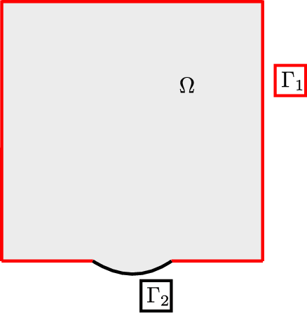
Quasi-absorbing boundary conditions are assumed for part of the boundary of the domain \(\Gamma_1\), as presented with red line in Figure 1, defined as

\[ \begin{align} \label{eq:two} \dfrac{\partial P({\mathbf{x}}, t)}{\partial t} + c\left({\mathbf{N}} \cdot \nabla P ({\mathbf{x}}, t) \right) = 0 \quad \text{on } \Gamma_1 \end{align} \]

where \(\mathbf{N}\) is the unit normal vector on the quasi absorbing boundary, \(\Gamma_1\).

A source of constant frequency, \(\omega\), and amplitude is assumed to be located on a different part of the boundary of the domain \(\Gamma_2\):

\[ \begin{align} \label{eq:three} P({\mathbf{x}}, t) = {\rm {cos}}(\omega t) \quad \text{on } \Gamma_2 \end{align} \]

where \(\Gamma_1\) is presented with black line in Figure 1,

Since we focus attention on a single frequency, we solve the problem in the frequency domain, reducing problem complexity. Assuming that the solution can admit variable separation:

\[ \begin{align} \label{eq:four} P({\mathbf{x}}, t) = {\rm Re}({p(\mathbf{x}) e^{-i \omega t} }) \end{align} \]

where now the spatially varying pressure amplitude, \(p(\mathbf{x})\), a complex value:

\[ \begin{align} \label{eq:five} p({\mathbf{x}}) = p^{\rm{Re}} + i p^{\rm{Im}} \end{align} \]

By introducing the wave number \(k = \omega / c \) and substituting \eqref{eq:four} and \eqref{eq:five} in \eqref{eq:one} to \eqref{eq:three} we arrive to the Helmholtz problem:

\[ \begin{equation} \begin{aligned} \newenvironment{rcases} {\left.\begin{aligned}} {\end{aligned}\right\rbrace} \begin{rcases} k^2 p^{\rm {Re}} + {\nabla}^2 p^{\rm {Re}} = 0 \\ k^2 p^{\rm {Im}} + {\nabla}^2 p^{\rm {Im}} = 0 \\ \end{rcases} {\text {in }} \Omega,\quad \newenvironment{rcases} {\left.\begin{aligned}} {\end{aligned}\right\rbrace} \begin{rcases} \mathbf{N} \cdot \nabla p^{\rm {Re}} + k p^{\rm {Im}} = 0 \\ \mathbf{N} \cdot \nabla p^{\rm {Im}} - k p^{\rm {Re}} = 0 \\ \end{rcases} {\text {on }} \Gamma_1,\quad \newenvironment{rcases} {\left.\begin{aligned}} {\end{aligned}\right\rbrace} \begin{rcases} p^{\rm {Re}} = 1 \\ p^{\rm {Im}} = 0 \\ \end{rcases} {\text {on }} \Gamma_2 \label{eq:six} \end{aligned} \end{equation} \]

It can be observed that the imaginary number \(i\) has disappeared since one can operate on the real and imaginary parts of the equation separately to fullfil an equation that is equal to zero. Therefore, the original problem of a single field, \( P({\mathbf{x}}, t) \), into a two field problem where one field is \(p^{\rm {Re}}\) and the second one \(p^{\rm {Re}}\).

The weak form and its discretisation

In this section the weak formulation is going to be presented and then extended to the equivalent discrete formulation. The weak formulation reads as this:

Find \( p^{\rm {Re}}\) and \(p^{\rm {Re}} \in H^1(\Omega) \) such that:

\[ \begin{equation} \begin{aligned} \label{eq:seven} \newenvironment{rcases} {\left.\begin{aligned}} {\end{aligned}\right\rbrace} \begin{rcases} k^2 {\int_{\Omega}} p^{\rm {Re}}\delta p^{\rm {Re}} {\rm d} {\Omega}+ {\int_{\Omega}}{\nabla}^2 p^{\rm {Re}} \delta p^{\rm {Re}}{\rm d} {\Omega} = 0 \\ k^2 {\int_{\Omega}} p^{\rm {Im}} \delta p^{\rm {Im}} {\rm d} {\Omega}+ {\int_{\Omega}}{\nabla}^2 p^{\rm {Im}}\delta p^{\rm {Im}}{\rm d} {\Omega} = 0 \\ \end{rcases} {\text {in }} \Omega,\quad \forall \delta p^{\rm {Re}}, \delta p^{\rm {Im}} \in H^1_0(\Omega)\\ \newenvironment{rcases} {\left.\begin{aligned}} {\end{aligned}\right\rbrace} \begin{rcases} {\int_{\Gamma_1}}\mathbf{N} \cdot \nabla p^{\rm {Re}} \delta p^{\rm {Re}} {\rm d} {\Gamma_1}+ {\int_{\Gamma_1}}k p^{\rm {Im}} \delta p^{\rm {Re}} {\rm d} {\Gamma_1}= 0 \\ {\int_{\Gamma_1}}\mathbf{N} \cdot \nabla p^{\rm {Im}} \delta p^{\rm {Im}} {\rm d} {\Gamma_1} - {\int_{\Gamma_1}}k p^{\rm {Re}} \delta p^{\rm {Im}} {\rm d} {\Gamma_1}= 0 \\ \end{rcases} {\text {on }} \Gamma_1,\quad \forall \delta p^{\rm {Re}}, \delta p^{\rm {Im}} \in H^1_0(\Omega)\\ \newenvironment{rcases} {\left.\begin{aligned}} {\end{aligned}\right\rbrace} \begin{rcases} {\int_{\Gamma_2}}p^{\rm {Re}} \delta p^{\rm {Re}} {\rm d} {\Gamma_2}= {\int_{\Gamma_2}}\delta p^{\rm {Re}} {\rm d} {\Gamma_2} \\ p^{\rm {Im}} = 0 \\ \end{rcases} {\text {on }} \Gamma_2,\quad \forall \delta p^{\rm {Re}}, \delta p^{\rm {Im}} \in H^1_0(\Omega) \end{aligned} \end{equation} \]

where \(\delta p^{\rm {Re}}\) and \(\delta p^{\rm {Im}}\) are the trial functions for the real and imaginary fields, respectively, and fulfil the identity, \( \delta p({\mathbf{x}}) = \delta p^{\rm {Re}} + i \delta p^{\rm {Im}}\).

By applying integration by parts for the laplacian term for the domain integral and substituting the

\[ \begin{equation} \begin{aligned} {p}^{\rm {Re}} \approx {p}^{h{\rm {Re}}} = \sum^{N-1}_{j = 0 } \phi_j {\bar {p}}^{\rm {Re}}_j, \quad {p}^{\rm {Im}} \approx {p}^{h{\rm {Im}}} = \sum^{N-1}_{j = 0 } \psi_j {\bar {p}}^{\rm {Im}}_j \label{eq:eight} \end{aligned} \end{equation} \]

the system of equations presented below are derived

\[ \begin{align} \label{eq:nine} \newenvironment{rcases} {\left.\begin{aligned}} {\end{aligned}\right\rbrace} \begin{rcases} \sum^{N-1}_{j = 0 } (k^2 {\displaystyle{\int_{\Omega}}} \phi_i \phi_j {\rm{d}}\Omega - {\int_{\Omega}} \nabla \phi_i \nabla\phi_j {\rm{d}}\Omega) {\bar p}^{\rm{Re}}_j - k ({\displaystyle{\int_{\Gamma_1}}} \phi_i\psi_j {\rm{d}}\Gamma_1) {\bar p}^{\rm{Im}}_j = 0 \\ \sum^{N-1}_{j = 0 } (k^2 {\displaystyle{\int_{\Omega}}} \psi_i \psi_j {\rm{d}}\Omega - {\int_{\Omega}} \nabla \psi_i \nabla\psi_j {\rm{d}}\Omega) {\bar p}^{\rm{Im}}_j + k ({\displaystyle{\int_{\Gamma_1}}} \psi_i\phi_j {\rm{d}}\Gamma_1) {\bar p}^{\rm{Re}}_j = 0 \\ \end{rcases} \quad \forall i = 0, .... (N-1) \end{align} \]

after grouping the unknowns and their coefficients the matrix notation is obtained:

\[ \begin{align} \label{eq:ten} \left[ \begin{array}{c c} k^2 {\displaystyle{\int_{\Omega}}} \phi_i \phi_j {\rm{d}}\Omega - {\int_{\Omega}} \nabla \phi_i \nabla\phi_j {\rm{d}}\Omega & -k {\displaystyle{\int_{\Gamma_1}}} \phi_i\psi_j {\rm{d}}\Gamma_1 \\ \\ k{\displaystyle{\int_{\Gamma_1}}} \psi_i\phi_j {\rm{d}}\Gamma_1 & + k^2 \displaystyle{{\int_{\Omega}}} \psi_i \psi_j {\rm{d}}\Omega - \displaystyle{{\int_{\Omega}}} \nabla \psi_i \nabla\psi_j {\rm{d}}\Omega \end{array} \right] \left[ \begin{array}{c} {\bar {p}}^{\rm {Re}}_j \\[0.2cm] {\bar {p}}^{\rm {Im}}_j \end{array} \right] = \left[ \begin{array}{c} \mathbf 0 \\ \mathbf 0 \end{array} \right] \end{align} \]

And essential boundary conditions applied on \(\Gamma_2\) are after applying discretisation are

\[ \begin{align} \label{eq:eleven} \sum^{N-1}_{j = 0 } -\left({\displaystyle{\int_{\Gamma_2}}} \phi_i \phi_j {\rm{d}}\Gamma_2\right){\bar{p^{\rm{Re}}_j}} = -{\displaystyle{\int_{\Gamma_2}}} \phi_i {\rm{d}}\Gamma_2 \quad \forall i = 0,...(N-1) \end{align} \]

Implementation

The focus of this section is on describing the procedure for solving two field problems in MoFEM using interface MoFEM::Simple, determining boundary conditions, using boundary and domain elements accessed through the interface and pushing form integrators to pipelines for solving the problem.

Declaration of fields for solution

The focus of this section is on the points highlighted in the Notes in the beginning of the tutorial. The problem is run by execution of a series of functions when invoking the function Example::runProblem():

where Example::readMesh() executes the mesh reading procedure, then Example::setupProblem() involves adding the two unknown fields on the entities of the mesh and determine the base function space, base, field rank and base order

// Add field
CHKERR simpleInterface->addDomainField("P_REAL", H1,
CHKERR simpleInterface->addDomainField("P_IMAG", H1,
CHKERR simpleInterface->addBoundaryField("P_REAL", H1,
CHKERR simpleInterface->addBoundaryField("P_IMAG", H1,
int order = 6;
CHKERR PetscOptionsGetInt(PETSC_NULL, "", "-order", &order, PETSC_NULL);
CHKERR simpleInterface->setFieldOrder("P_REAL", order);
CHKERR simpleInterface->setFieldOrder("P_IMAG", order);
}

where the fields \(p^{\rm{Re}}\) and \(p^{\rm{Im}}\) are marked as P_REAL and P_IMAG, respectively. Furthermore, the space chosen is H1, the base is AINSWORTH_BERNSTEIN_BEZIER_BASE and dimension is 1 that corresponds to a scalar field. The field data is added both to Domain Element and Boundary Element from Simple Interface via invoking addDomainField and addBoundaryField, respectively. As it will be shown later, for a problem solved in \(\mathbb{R}^d\) where \( d \) is the problem dimension, Domain Elements perform operations on the mesh entities of the highest dimension ( \(\mathbb{R}^d\)) and Boundary Elements that perform operations on mesh entities of dimension \( d - 1\) that lie only on the boundary of the mesh, in this case \( \Gamma_1\) and \( \Gamma_2\).

Moreover, the base functions corresponding to \(p^{\rm{Re}}\) and to \(p^{\rm{Im}}\)

CHKERR simpleInterface->setFieldOrder("P_REAL", order);
CHKERR simpleInterface->setFieldOrder("P_IMAG", order);

where the default value is set to be 6

int order = 6;

and can be changed by determining the order of choice via the command line parameter -order. Finally, the fields are set up via simpleInterface->setUp().

Boundary treatment

Thereafter, the boundary entities are marked based on the input in Example::boundaryCondition() as shown in the snippet below

auto get_ents_on_mesh_skin = [&]() {
Range boundary_entities;
std::string entity_name = it->getName();
if (entity_name.compare(0, 2, "BC") == 0) {
CHKERR it->getMeshsetIdEntitiesByDimension(mField.get_moab(), 1,
boundary_entities, true);
}
}
// Add vertices to boundary entities
Range boundary_vertices;
CHKERR mField.get_moab().get_connectivity(boundary_entities,
boundary_vertices, true);
boundary_entities.merge(boundary_vertices);
return boundary_entities;
};
auto mark_boundary_dofs = [&](Range &&skin_edges) {
auto problem_manager = mField.getInterface<ProblemsManager>();
auto marker_ptr = boost::make_shared<std::vector<unsigned char>>();
problem_manager->markDofs(simpleInterface->getProblemName(), ROW,
skin_edges, *marker_ptr);
return marker_ptr;
};
auto remove_dofs_from_problem = [&](Range &&skin_edges) {
auto problem_manager = mField.getInterface<ProblemsManager>();
CHKERR problem_manager->removeDofsOnEntities(
simpleInterface->getProblemName(), "P_IMAG", skin_edges, 0, 1);
};
// Get global local vector of marked DOFs. Is global, since is set for all
// DOFs on processor. Is local since only DOFs on processor are in the
// vector. To access DOFs use local indices.
boundaryMarker = mark_boundary_dofs(get_ents_on_mesh_skin());
CHKERR remove_dofs_from_problem(get_ents_on_mesh_skin());
}

The present code is designated for 2D problems. Hence, all vertices and edges located on the \(\Gamma_2\) boundary, marked with BLOCK_SET with name "BC" in the input file, are added to the global variable Example::boundaryMarker that will be used in the assembly procedure. Furthermore, due to uniform essential boundary conditions on \(\Gamma_2\) for the Imaginary field, the dofs located on that boundary are deleted from the problem via the lambda function remove_dofs_from_problem.

Pushing UDOs to domain and boundary pipelines

Function Example::assembleSystem() is responsible for evaluating linear and bilinear forms for the problem and assembling the system to be solved

PipelineManager *pipeline_mng = mField.getInterface<PipelineManager>();
double k = 90;
CHKERR PetscOptionsGetScalar(PETSC_NULL, "", "-k", &k, PETSC_NULL);
auto beta = [](const double, const double, const double) { return -1; };
auto k2 = [k](const double, const double, const double) { return pow(k, 2); };
auto kp = [k](const double, const double, const double) { return k; };
auto km = [k](const double, const double, const double) { return -k; };
auto integration_rule = [](int, int, int p_data) { return 2 * p_data; };
auto set_domain = [&]() {
CHKERR AddHOOps<SPACE_DIM, SPACE_DIM, SPACE_DIM>::add(
pipeline_mng->getOpDomainLhsPipeline(), {H1});
pipeline_mng->getOpDomainLhsPipeline().push_back(
new OpSetBc("P_REAL", true, boundaryMarker));
pipeline_mng->getOpDomainLhsPipeline().push_back(
new OpDomainGradGrad("P_REAL", "P_REAL", beta));
pipeline_mng->getOpDomainLhsPipeline().push_back(
new OpDomainGradGrad("P_IMAG", "P_IMAG", beta));
pipeline_mng->getOpDomainLhsPipeline().push_back(
new OpDomainMass("P_REAL", "P_REAL", k2));
pipeline_mng->getOpDomainLhsPipeline().push_back(
new OpDomainMass("P_IMAG", "P_IMAG", k2));
pipeline_mng->getOpDomainLhsPipeline().push_back(new OpUnSetBc("P_REAL"));
CHKERR pipeline_mng->setDomainLhsIntegrationRule(integration_rule);
};
auto set_boundary = [&]() {
CHKERR AddHOOps<SPACE_DIM - 1, SPACE_DIM, SPACE_DIM>::add(
pipeline_mng->getOpBoundaryLhsPipeline(), {});
pipeline_mng->getOpBoundaryLhsPipeline().push_back(
new OpSetBc("P_REAL", true, boundaryMarker));
pipeline_mng->getOpBoundaryLhsPipeline().push_back(
new OpBoundaryMass("P_IMAG", "P_REAL", kp));
pipeline_mng->getOpBoundaryLhsPipeline().push_back(
new OpBoundaryMass("P_REAL", "P_IMAG", km));
pipeline_mng->getOpBoundaryLhsPipeline().push_back(new OpUnSetBc("P_REAL"));
pipeline_mng->getOpBoundaryLhsPipeline().push_back(
new OpSetBc("P_REAL", false, boundaryMarker));
pipeline_mng->getOpBoundaryLhsPipeline().push_back(
new OpBoundaryMass("P_REAL", "P_REAL", beta));
pipeline_mng->getOpBoundaryLhsPipeline().push_back(new OpUnSetBc("P_REAL"));
pipeline_mng->getOpBoundaryRhsPipeline().push_back(
new OpSetBc("P_REAL", false, boundaryMarker));
pipeline_mng->getOpBoundaryRhsPipeline().push_back(
new OpBoundarySource("P_REAL", beta));
pipeline_mng->getOpBoundaryRhsPipeline().push_back(new OpUnSetBc("P_REAL"));
CHKERR pipeline_mng->setBoundaryRhsIntegrationRule(integration_rule);
CHKERR pipeline_mng->setBoundaryLhsIntegrationRule(integration_rule);
};
CHKERR set_domain();
CHKERR set_boundary();
}

where the wave-number \(k\) has a default value of 90 and can be determined by the user via command line option -k as dictated by the lines below

double k = 90;
CHKERR PetscOptionsGetScalar(PETSC_NULL, "", "-k", &k, PETSC_NULL);

Thereafter, five lambda functions are determined

auto beta = [](const double, const double, const double) { return -1; };
auto k2 = [k](const double, const double, const double) { return pow(k, 2); };
auto kp = [k](const double, const double, const double) { return k; };
auto km = [k](const double, const double, const double) { return -k; };

that are going to be used as pointer functions in the rest of the function and explained in more detail later.

Moreover, in Example::assembleSystem() operators are pushed to different pipelines managed by the common Pipe Line object pipeline_mng

getOpDomainLhsPipeline()
getOpBoundaryLhsPipeline()
getOpBoundaryRhsPipeline()

when operators are pushed by invoking getOpDomainLhsPipeline(), they will be set to be operating on Domain elements and assembling on the LHS of the system of equations. When operators are pushed by invoking getOpBoundaryLhsPipeline() and getOpBoundaryRhsPipeline(), they will be set to be operating on Boundary elements and assembling on the LHS and RHS, respectively.

Two lambda functions set_domain and set_boundary are dedicated to push operators to Domain and Boundary pipelines respectively.

Pushing operators to LHS domain pipeline

In set_domain lambda function, operators are pushed only in Domain LHS Pipeline. For 2D elements, such as those used in the present tutorial, a pre-processing operation has to be applied to evaluate the gradient of the shape functions. For this, the operators below have to be pushed.

auto det_ptr = boost::make_shared<VectorDouble>();
auto jac_ptr = boost::make_shared<MatrixDouble>();
auto inv_jac_ptr = boost::make_shared<MatrixDouble>();
pipeline_mng->getOpDomainLhsPipeline().push_back(new OpCalculateHOJacForFace(jac_ptr));
pipeline_mng->getOpDomainLhsPipeline().push_back(new OpInvertMatrix<2>(jac_ptr, det_ptr, inv_jac_ptr));
pipeline_mng->getOpDomainLhsPipeline().push_back(
new OpSetHOInvJacToScalarBases<2>(H1, inv_jac_ptr));
pipeline_mng->getOpDomainLhsPipeline().push_back(new OpSetHOWeightsOnFace());

where the first operator evaluates the inverse of the Jacobian at each gauss point. Then, this variable is passed to the second operator and for each gauss point the gradient of the shape function is multiplied with the inverse of the Jacobian so that these gradient correspond to the spatial configuration of the element rather than the parent according to the relationship below

\[ \begin{equation} \begin{aligned} (\nabla \phi)_j = \dfrac{\partial \phi}{\partial \xi_i} \dfrac{\partial \xi_{i}}{\partial X_j} \label{eq:twelve} \end{aligned} \end{equation} \]

where \(\xi_i\) are the parent coordinates \(X_j\) are the global coordinates at the gauss point of interest.

Next, the operator pushed is related to treatment of degrees of freedom located at the boundary \(\Gamma_2\) where Essential boundary conditions are applied since the global variable Example::boundaryMarker is passed where all entities located on \(\Gamma_2\) are stored.

pipeline_mng->getOpDomainLhsPipeline().push_back(
new OpSetBc("P_REAL", true, boundaryMarker));

This operator acts on dofs of \(p^{\rm{Re}}\) since string "P_REAL" is passed. By pushing this operator with flag true, all indices that correspond to the dofs corresponding to entities in Example::boundaryMarker that lie on the boundary are set to -1. This will prevent the next operators to assemble the stiffness matrix to rows-columns combination corresponding to those dofs. If flag false was chosen, all the indices corresponding to dofs corresponding to entities located to all the boundary except those in Example::boundaryMarker would be set to -1.

Thereafter, bilinear forms for gradients for \(p^{\rm{Re}}\) and \(p^{\rm{Im}}\) as shown at the two diagonal sub-matrices in \eqref{eq:ten}

\[ \begin{align} \label{eq:thirteen} -{\int_{\Omega}} \nabla \phi_i \nabla\phi_j {\rm{d}}\Omega,\quad -{\int_{\Omega}} \nabla \psi_i \nabla\psi_j {\rm{d}}\Omega \end{align} \]

are evaluated by pushing the next two Operators

pipeline_mng->getOpDomainLhsPipeline().push_back(
new OpDomainGradGrad("P_REAL", "P_REAL", beta));
pipeline_mng->getOpDomainLhsPipeline().push_back(
new OpDomainGradGrad("P_IMAG", "P_IMAG", beta));

where for the first and second push correspond to the first and second integral presented in \eqref{eq:thirteen}. Moreover, OpDomainGradGrad stands for an alias for the OpGradGrad template specialisation

using OpDomainGradGrad = FormsIntegrators<DomainEleOp>::Assembly<

determined in the beginning of the file, where DomainEleOp is also an alias for User Data Operator from Face Elements also determined in the beginning of the file as

Furthermore, the lambda function beta that returns -1 is passed as pointer function so that it will multiply the integral such that it will be assembled with the negative sign as shown in \eqref{eq:thirteen}.

Thereafter, the operator OpDomainMass is pushed twice to the domain LHS pipeline

pipeline_mng->getOpDomainLhsPipeline().push_back(
new OpDomainMass("P_REAL", "P_REAL", k2));
pipeline_mng->getOpDomainLhsPipeline().push_back(
new OpDomainMass("P_IMAG", "P_IMAG", k2));

where the first push operates on \(p^{\rm{Re}}\) rows and cols and the second push operates on \(p^{\rm{Re}}\) rows and cols. These operators will be used from the domain element when the solver will invoke the pipeline to evaluate the mass matrices located on the diagonal sub-matrices in \eqref{eq:ten}

\[ \begin{align} \label{eq:fourteen} k^2{\int_{\Omega}} \phi_i \phi_j {\rm{d}}\Omega,\quad k^2{\int_{\Omega}} \psi_i \psi_j {\rm{d}}\Omega \end{align} \]

Also, the OpDomainMass is an alias of the specialisation of the form integrator template OpMass declared in the beginning of the file

using OpDomainMass = FormsIntegrators<DomainEleOp>::Assembly<

that is of element operator type DomainEleOp similar to the OpDomainGradGrad form integrator shown before. Moreover, in both pushes of OpDomainMass, the lambda function k2, that returns the input of square of wave-number \(k\), is passed as pointer function in order to multiply the mass matrix by \(k^2\) as shown in \eqref{eq:fourteen}.

After all form integrators have been pushed to the Domain LHS pipeline, the dofs that were marked in order not to be used located on \(\Gamma_2\) so that the next pipeline will receive the dofs conditioning in its virgin configuration. This is achieved by pushing operator OpUnSetBc as

pipeline_mng->getOpDomainLhsPipeline().push_back(new OpUnSetBc("P_REAL"));

At the end of lambda function set_domain, the integration rule for the Domain element for LHS is determined as

CHKERR pipeline_mng->setDomainLhsIntegrationRule(integration_rule);
\code
where lambda function `integration_rule` is passed as pointer function that has access to the order of the field under consideration and sets the rule to twice the order as shown below
\code
auto integration_rule = [](int, int, int p_data) { return 2 * p_data; };

Pushing operators to LHS and RHS boundary pipeline

In set_boundary lambda function, operators are pushed to the Boundary LHS and RHS pipelines. Initially, for LHS Boundary pipeline the dofs corresponding to entities contained in Example::boundaryMarker Range variable for \(p^{\rm{Re}}\) (located on the \(\Gamma_2\) boundary) are marked not to allow any assembly of the bilinear forms pushed in the pipeline.

pipeline_mng->getOpBoundaryLhsPipeline().push_back(
new OpSetBc("P_REAL", true, boundaryMarker));

Thereafter, the mass matrix type bilinear form integrated on \(\Gamma_1\) boundary

pipeline_mng->getOpBoundaryLhsPipeline().push_back(
new OpBoundaryMass("P_IMAG", "P_REAL", kp));

that corresponds to imaginary rows and real columns ("P_IMAG", "P_REAL") presented in \eqref{eq:ten} and given by the formula

\[ \begin{align} \label{eq:fifteen} k{\int_{\Gamma_1}} \psi_i \phi_j {\rm{d}}\Gamma_1 \end{align} \]

where lambda function kp is passed as pointer function to multiply the bilinear form by \(k\) as shown in \eqref{eq:fifteen}. Operator OpBoundaryMass is an alias of bilinear form template specialisation, OpMass, determined in the top of the file as

using OpBoundaryMass = FormsIntegrators<EdgeEleOp>::Assembly<

where the difference with the alias operator previously presented, OpDomainMass, is that the present template specialisation acts on the boundary element operator , EdgeEleOp, determined also at the top of the file as

The next operator push is the same, OpBoundaryMass, that now acts on the real rows and imaginary columns

pipeline_mng->getOpBoundaryLhsPipeline().push_back(
new OpBoundaryMass("P_REAL", "P_IMAG", km));

that evaluates and assembles the bilinear form

\[ \begin{align} \label{eq:sixteen} -k{\int_{\Gamma_1}} \phi_i \psi_j {\rm{d}}\Gamma_1 \end{align} \]

as shown in \eqref{eq:ten} and lambda function km is passed in order to multiply \(-k\) as presented in \eqref{eq:sixteen}. Once all the operators for the Boundary LHS pipeline operating on \(\Gamma_1\) are pushed, the marked dofs have to be release so that the dofs conditioning will be passed intact to the next pipeline and achieved by pushing OpUnSetBc

pipeline_mng->getOpBoundaryLhsPipeline().push_back(new OpUnSetBc("P_REAL"));

Essential boundary conditions are also applied following \eqref{eq:eleven} but assumed to have both side multiplied by -1. Initially, operator OpSetBc is now used by setting false flag so that now the rest of the boundary except for \(\Gamma_2\) is now marked not to allow for assembly as

pipeline_mng->getOpBoundaryLhsPipeline().push_back(
new OpSetBc("P_REAL", false, boundaryMarker));

Then the mass bilinear form integrator is pushed using beta lambda function to multiply the integral by -1.

pipeline_mng->getOpBoundaryLhsPipeline().push_back(
new OpBoundaryMass("P_REAL", "P_REAL", beta));

and then the marked boundary is released again by

pipeline_mng->getOpBoundaryLhsPipeline().push_back(new OpUnSetBc("P_REAL"));

For setting the RHS linear form the boundary is appropriately marked as in the case for the bilinear form corresponding to the essential boundary conditions but now for the Boundary RHS pipeline as

pipeline_mng->getOpBoundaryRhsPipeline().push_back(
new OpSetBc("P_REAL", false, boundaryMarker));

then the linear form is pushed with lambda function beta so that the integral presented in the RHS in \eqref{eq:eleven} is multiplied by -1

pipeline_mng->getOpBoundaryRhsPipeline().push_back(
new OpBoundarySource("P_REAL", beta));

where operator OpBoundarySource is an alias of the template specialisation OpSource assigned in the beginning of the file

using OpBoundarySource = FormsIntegrators<EdgeEleOp>::Assembly<
PETSC>::LinearForm<GAUSS>::OpSource<1, 1>;

and then marked boundary dofs are released again

pipeline_mng->getOpBoundaryRhsPipeline().push_back(new OpUnSetBc("P_REAL"));

Finally, integration rules are set for RHS and LHS for Boundary element.

CHKERR pipeline_mng->setBoundaryRhsIntegrationRule(integration_rule);
CHKERR pipeline_mng->setBoundaryLhsIntegrationRule(integration_rule);

Solving and outputting results

The last three functions invoked in Example::runProblem() are

CHKERR solveSystem();
CHKERR outputResults();
CHKERR checkResults();

that each involve solving the system of linear equations using KSPSolver, printing the results for the two fields P_REAL and P_IMAG and checking convergence of the system respectively.

The implementation of these three functions is not discussed in the present tutorial as it is not the focus as discussed in the notes in the beginning of the tutorial. Description of such functions will be discussed in other tutorials.

Running the code and post processing

In order to run the program that we have been discussing in this tutorial, you will have to follow the steps below

  • First, move to the directory where the binary file helmholtz is located. Depending on how you install MoFEM shown in this page Installation with Spack (Scripts), going to the directory would be something similar to this
    • For user version installation
      cd mofem_install/um_view/tutorials/clx-0/
    • For developer version installation
      cd mofem_install/um/build_release/tutorials/clx-0/
  • Second, check the parameters in the param_file.petsc. These are PETSc parameters and you should only use parameters that are needed for a particular solver, in this case KSP solver. Only the following parameters should be uncommented
    ## Linear solver
    -pc_type lu
    -pc_factor_mat_solver_type mumps
    -ksp_monitor
  • Third, in the terminal, run commands to partition the input mesh and start the analysis
    mofem_part -my_file geometry.cub -output_file part.h5m -my_nparts 2 -dim 2 -adj_dim 1
    mpirun -np 2 ./helmholtz -file_name part.h5m -order 8 -k 180
    where in the first line the mesh geometry.cub presented in Figure 2 generated in the open source code CUBIT is partitioned in to parts and generated the partitioned mesh part.h5m with boundaries and domain corresponding to \(Gamma_1\) and \(Gamma_2\) presented in Figure 1. In the second line, program is run using two processors (the same number of partitions) with fourth order polynomial of approximation and \(k = 90\).

Figure 2: Mesh under the name `geometry.cub` used for partitioning.
  • After the analysis has run successfully, an output file, out_helmholtz.h5m, is generated. To convert the results from .h5m format into .vtk
    mbconvert out_helmholtz.h5m out_helmholtz.vtk
  • To evaluate the wave amplitude from the results, once the out_helmholtz.vtk file is openned in freely available postprocessing software the calculator solver must be used to evaluate from the solution of the fields P_REAL and P_IMAG by setting the name Intensity in the Result Array Name field and calculating the wave amplitude as \(\sqrt{\left(p^{\rm{Re}}\right)^2 + \left(p^{\rm{Im}}\right)^2}\) by substituting
    sqrt(P_REAL* P_REAL+P_IMAG*P_IMAG)
    into the field below Result Array Name. The associated results are presented in Figure 3.

Figure 3: Post processed results for intensity (magnitude) of the result for wave-number 180 and order for approximation shape functions.
  • Finally to obtain a series of files to resemble the evolution in time of the stationary wave evaluated one has to paste the code below to the python shell of paraview
my_out = FindSource("out_helmholtz.vtk")
for t in range(100):
tt = 10*t / float(100)
calculator1 = Calculator(Input=my_out)
calculator1.Function = "P_REAL*cos(2*3.141* " + str(tt) + ") + P_IMAG*sin(2*3.141*" + str(tt) + ")"
passArrays1 = PassArrays(Input=calculator1)
passArrays1.PointDataArrays = ['new_array']
SaveData("./out_" + str(t) + ".vtk", proxy=passArrays1, FileType='Ascii')
Delete(calculator1)
Delete(passArrays1)

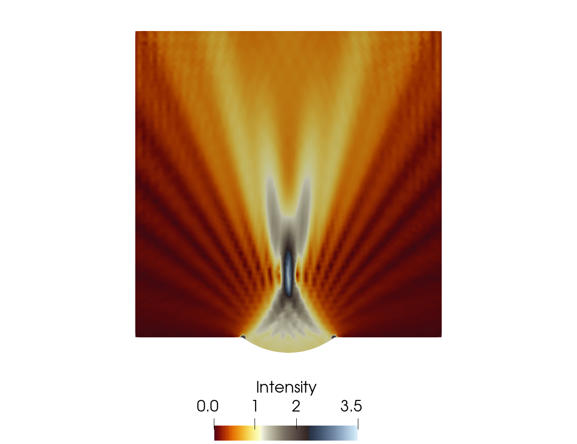
compiling the series of 100 files generated the video presented in Figure 4 will be generated

Figure 4: Post processed results for visual presentation of the periodic movement of the stationary wave corresponding to the solution of the Helmholtz problem in frequency domain.
/**
* \file helmholtz.cpp
* \example helmholtz.cpp
*
* Using PipelineManager interface calculate Helmholtz problem. Example show how
* to manage complex variable fields.
*/
#include <MoFEM.hpp>
using namespace MoFEM;
static char help[] = "...\n\n";
constexpr int SPACE_DIM = 2;
PETSC>::LinearForm<GAUSS>::OpSource<1, 1>;
struct Example {
Example(MoFEM::Interface &m_field) : mField(m_field) {}
MoFEMErrorCode runProblem();
private:
Simple *simpleInterface;
boost::shared_ptr<std::vector<unsigned char>> boundaryMarker;
MoFEMErrorCode readMesh();
MoFEMErrorCode setupProblem();
MoFEMErrorCode boundaryCondition();
MoFEMErrorCode assembleSystem();
MoFEMErrorCode solveSystem();
MoFEMErrorCode outputResults();
MoFEMErrorCode checkResults();
};
//! [run problem]
CHKERR readMesh();
CHKERR setupProblem();
CHKERR boundaryCondition();
CHKERR assembleSystem();
CHKERR solveSystem();
CHKERR outputResults();
CHKERR checkResults();
}
//! [run problem]
//! [Read mesh]
CHKERR mField.getInterface(simpleInterface);
CHKERR simpleInterface->getOptions();
CHKERR simpleInterface->loadFile();
}
//! [Read mesh]
//! [Set up problem]
// Add field
CHKERR simpleInterface->addDomainField("P_REAL", H1,
CHKERR simpleInterface->addDomainField("P_IMAG", H1,
CHKERR simpleInterface->addBoundaryField("P_REAL", H1,
CHKERR simpleInterface->addBoundaryField("P_IMAG", H1,
int order = 6;
CHKERR PetscOptionsGetInt(PETSC_NULL, "", "-order", &order, PETSC_NULL);
CHKERR simpleInterface->setFieldOrder("P_REAL", order);
CHKERR simpleInterface->setFieldOrder("P_IMAG", order);
CHKERR simpleInterface->setUp();
}
//! [Set up problem]
//! [Applying essential BC]
auto get_ents_on_mesh_skin = [&]() {
Range boundary_entities;
std::string entity_name = it->getName();
if (entity_name.compare(0, 2, "BC") == 0) {
CHKERR it->getMeshsetIdEntitiesByDimension(mField.get_moab(), 1,
boundary_entities, true);
}
}
// Add vertices to boundary entities
Range boundary_vertices;
CHKERR mField.get_moab().get_connectivity(boundary_entities,
boundary_vertices, true);
boundary_entities.merge(boundary_vertices);
return boundary_entities;
};
auto mark_boundary_dofs = [&](Range &&skin_edges) {
auto problem_manager = mField.getInterface<ProblemsManager>();
auto marker_ptr = boost::make_shared<std::vector<unsigned char>>();
problem_manager->markDofs(simpleInterface->getProblemName(), ROW,
skin_edges, *marker_ptr);
return marker_ptr;
};
auto remove_dofs_from_problem = [&](Range &&skin_edges) {
auto problem_manager = mField.getInterface<ProblemsManager>();
CHKERR problem_manager->removeDofsOnEntities(
simpleInterface->getProblemName(), "P_IMAG", skin_edges, 0, 1);
};
// Get global local vector of marked DOFs. Is global, since is set for all
// DOFs on processor. Is local since only DOFs on processor are in the
// vector. To access DOFs use local indices.
boundaryMarker = mark_boundary_dofs(get_ents_on_mesh_skin());
CHKERR remove_dofs_from_problem(get_ents_on_mesh_skin());
}
//! [Applying essential BC]
//! [Push operators to pipeline]
PipelineManager *pipeline_mng = mField.getInterface<PipelineManager>();
double k = 90;
CHKERR PetscOptionsGetScalar(PETSC_NULL, "", "-k", &k, PETSC_NULL);
auto beta = [](const double, const double, const double) { return -1; };
auto k2 = [k](const double, const double, const double) { return pow(k, 2); };
auto kp = [k](const double, const double, const double) { return k; };
auto km = [k](const double, const double, const double) { return -k; };
auto integration_rule = [](int, int, int p_data) { return 2 * p_data; };
auto set_domain = [&]() {
pipeline_mng->getOpDomainLhsPipeline(), {H1});
pipeline_mng->getOpDomainLhsPipeline().push_back(
new OpSetBc("P_REAL", true, boundaryMarker));
pipeline_mng->getOpDomainLhsPipeline().push_back(
new OpDomainGradGrad("P_REAL", "P_REAL", beta));
pipeline_mng->getOpDomainLhsPipeline().push_back(
new OpDomainGradGrad("P_IMAG", "P_IMAG", beta));
pipeline_mng->getOpDomainLhsPipeline().push_back(
new OpDomainMass("P_REAL", "P_REAL", k2));
pipeline_mng->getOpDomainLhsPipeline().push_back(
new OpDomainMass("P_IMAG", "P_IMAG", k2));
pipeline_mng->getOpDomainLhsPipeline().push_back(new OpUnSetBc("P_REAL"));
};
auto set_boundary = [&]() {
pipeline_mng->getOpBoundaryLhsPipeline(), {});
pipeline_mng->getOpBoundaryLhsPipeline().push_back(
new OpSetBc("P_REAL", true, boundaryMarker));
pipeline_mng->getOpBoundaryLhsPipeline().push_back(
new OpBoundaryMass("P_IMAG", "P_REAL", kp));
pipeline_mng->getOpBoundaryLhsPipeline().push_back(
new OpBoundaryMass("P_REAL", "P_IMAG", km));
pipeline_mng->getOpBoundaryLhsPipeline().push_back(new OpUnSetBc("P_REAL"));
pipeline_mng->getOpBoundaryLhsPipeline().push_back(
new OpSetBc("P_REAL", false, boundaryMarker));
pipeline_mng->getOpBoundaryLhsPipeline().push_back(
new OpBoundaryMass("P_REAL", "P_REAL", beta));
pipeline_mng->getOpBoundaryLhsPipeline().push_back(new OpUnSetBc("P_REAL"));
pipeline_mng->getOpBoundaryRhsPipeline().push_back(
new OpSetBc("P_REAL", false, boundaryMarker));
pipeline_mng->getOpBoundaryRhsPipeline().push_back(
new OpBoundarySource("P_REAL", beta));
pipeline_mng->getOpBoundaryRhsPipeline().push_back(new OpUnSetBc("P_REAL"));
};
CHKERR set_domain();
CHKERR set_boundary();
}
//! [Push operators to pipeline]
//! [Solve]
PipelineManager *pipeline_mng = mField.getInterface<PipelineManager>();
auto solver = pipeline_mng->createKSP();
CHKERR KSPSetFromOptions(solver);
CHKERR KSPSetUp(solver);
auto dm = simpleInterface->getDM();
auto D = createDMVector(dm);
auto F = vectorDuplicate(D);
CHKERR KSPSolve(solver, F, D);
CHKERR VecGhostUpdateBegin(D, INSERT_VALUES, SCATTER_FORWARD);
CHKERR VecGhostUpdateEnd(D, INSERT_VALUES, SCATTER_FORWARD);
CHKERR DMoFEMMeshToLocalVector(dm, D, INSERT_VALUES, SCATTER_REVERSE);
}
//! [Solve]
//! [Postprocess results]
PipelineManager *pipeline_mng = mField.getInterface<PipelineManager>();
pipeline_mng->getDomainLhsFE().reset();
pipeline_mng->getDomainRhsFE().reset();
pipeline_mng->getBoundaryLhsFE().reset();
pipeline_mng->getBoundaryRhsFE().reset();
auto post_proc_fe = boost::make_shared<PostProcEle>(mField);
auto p_real_ptr = boost::make_shared<VectorDouble>();
auto p_imag_ptr = boost::make_shared<VectorDouble>();
post_proc_fe->getOpPtrVector().push_back(
new OpCalculateScalarFieldValues("P_REAL", p_real_ptr));
post_proc_fe->getOpPtrVector().push_back(
new OpCalculateScalarFieldValues("P_IMAG", p_imag_ptr));
post_proc_fe->getOpPtrVector().push_back(
new OpPPMap(
post_proc_fe->getPostProcMesh(), post_proc_fe->getMapGaussPts(),
{{"P_REAL", p_real_ptr}, {"P_IMAG", p_imag_ptr}},
{}, {}, {}
)
);
pipeline_mng->getDomainRhsFE() = post_proc_fe;
CHKERR pipeline_mng->loopFiniteElements();
CHKERR post_proc_fe->writeFile("out_helmholtz.h5m");
}
//! [Postprocess results]
//! [Check results]
auto dm = simpleInterface->getDM();
auto D = createDMVector(dm);
CHKERR DMoFEMMeshToLocalVector(dm, D, INSERT_VALUES, SCATTER_FORWARD);
double nrm2;
CHKERR VecNorm(D, NORM_2, &nrm2);
MOFEM_LOG("WORLD", Sev::inform)
<< std::setprecision(9) << "Solution norm " << nrm2;
PetscBool test_flg = PETSC_FALSE;
CHKERR PetscOptionsGetBool(PETSC_NULL, "", "-test", &test_flg, PETSC_NULL);
if (test_flg) {
constexpr double regression_test = 97.261672;
constexpr double eps = 1e-6;
if (std::abs(nrm2 - regression_test) / regression_test > eps)
SETERRQ(PETSC_COMM_SELF, MOFEM_DATA_INCONSISTENCY,
"Not converged solution");
}
}
//! [Check results]
int main(int argc, char *argv[]) {
// Initialisation of MoFEM/PETSc and MOAB data structures
const char param_file[] = "param_file.petsc";
MoFEM::Core::Initialize(&argc, &argv, param_file, help);
try {
//! [Register MoFEM discrete manager in PETSc]
DMType dm_name = "DMMOFEM";
//! [Register MoFEM discrete manager in PETSc
//! [Create MoAB]
moab::Core mb_instance; ///< mesh database
moab::Interface &moab = mb_instance; ///< mesh database interface
//! [Create MoAB]
//! [Create MoFEM]
MoFEM::Core core(moab); ///< finite element database
MoFEM::Interface &m_field = core; ///< finite element database insterface
//! [Create MoFEM]
//! [Example]
Example ex(m_field);
CHKERR ex.runProblem();
//! [Example]
}
}
MoFEM::UnknownInterface::getInterface
MoFEMErrorCode getInterface(IFACE *&iface) const
Get interface refernce to pointer of interface.
Definition: UnknownInterface.hpp:93
MoFEM::EdgeElementForcesAndSourcesCore
Edge finite element.
Definition: EdgeElementForcesAndSourcesCore.hpp:30
Example::checkResults
MoFEMErrorCode checkResults()
[Postprocess results]
Definition: dynamic_first_order_con_law.cpp:1205
MoFEM::PipelineManager::getDomainRhsFE
boost::shared_ptr< FEMethod > & getDomainRhsFE()
Definition: PipelineManager.hpp:405
Example::assembleSystem
MoFEMErrorCode assembleSystem()
[Push operators to pipeline]
Definition: dynamic_first_order_con_law.cpp:647
MoFEM::CoreTmp< 0 >
Core (interface) class.
Definition: Core.hpp:82
Example::boundaryMarker
boost::shared_ptr< std::vector< unsigned char > > boundaryMarker
Definition: helmholtz.cpp:42
H1
@ H1
continuous field
Definition: definitions.h:85
EdgeElementForcesAndSourcesCore
MoFEM::ProblemsManager
Problem manager is used to build and partition problems.
Definition: ProblemsManager.hpp:21
MoFEM::PipelineManager::loopFiniteElements
MoFEMErrorCode loopFiniteElements(SmartPetscObj< DM > dm=nullptr)
Iterate finite elements.
Definition: PipelineManager.cpp:19
paraview_deform_macro.Function
Function
Definition: paraview_deform_macro.py:15
help
static char help[]
Definition: activate_deactivate_dofs.cpp:13
MoFEM::Exceptions::MoFEMErrorCode
PetscErrorCode MoFEMErrorCode
MoFEM/PETSc error code.
Definition: Exceptions.hpp:56
MoFEM::PipelineManager::getBoundaryLhsFE
boost::shared_ptr< FEMethod > & getBoundaryLhsFE()
Definition: PipelineManager.hpp:409
Example::simpleInterface
Simple * simpleInterface
Definition: helmholtz.cpp:41
MoFEM::PETSC
@ PETSC
Definition: FormsIntegrators.hpp:104
MoFEM::PipelineManager
PipelineManager interface.
Definition: PipelineManager.hpp:24
MoFEM.hpp
MoFEM::DMoFEMMeshToLocalVector
PetscErrorCode DMoFEMMeshToLocalVector(DM dm, Vec l, InsertMode mode, ScatterMode scatter_mode)
set local (or ghosted) vector values on mesh for partition only
Definition: DMMoFEM.cpp:527
BasicFiniteElements.hpp
MoFEM::PipelineManager::getBoundaryRhsFE
boost::shared_ptr< FEMethod > & getBoundaryRhsFE()
Definition: PipelineManager.hpp:413
MoFEM::CoreTmp< 0 >::Finalize
static MoFEMErrorCode Finalize()
Checks for options to be called at the conclusion of the program.
Definition: Core.cpp:112
MoFEM::Simple
Simple interface for fast problem set-up.
Definition: Simple.hpp:27
paraview_deform_macro.calculator1
calculator1
Definition: paraview_deform_macro.py:12
OpDomainMass
FormsIntegrators< DomainEleOp >::Assembly< PETSC >::BiLinearForm< GAUSS >::OpMass< 1, FIELD_DIM > OpDomainMass
Definition: child_and_parent.cpp:53
order
constexpr int order
Definition: dg_projection.cpp:18
MoFEM::DeprecatedCoreInterface
Deprecated interface functions.
Definition: DeprecatedCoreInterface.hpp:16
OpBoundaryMass
FormsIntegrators< BoundaryEleOp >::Assembly< PETSC >::BiLinearForm< GAUSS >::OpMass< 1, SPACE_DIM > OpBoundaryMass
[Only used with Hencky/nonlinear material]
Definition: seepage.cpp:71
ROW
@ ROW
Definition: definitions.h:123
MoFEM::PipelineManager::getOpBoundaryLhsPipeline
boost::ptr_deque< UserDataOperator > & getOpBoundaryLhsPipeline()
Get the Op Boundary Lhs Pipeline object.
Definition: PipelineManager.hpp:797
MoFEM::Interface
DeprecatedCoreInterface Interface
Definition: Interface.hpp:1975
Example::readMesh
MoFEMErrorCode readMesh()
[Run problem]
Definition: dynamic_first_order_con_law.cpp:463
MoFEM::PostProcBrokenMeshInMoab
Definition: PostProcBrokenMeshInMoabBase.hpp:667
MoFEM::Simple::getDM
MoFEMErrorCode getDM(DM *dm)
Get DM.
Definition: Simple.cpp:667
CHKERR
#define CHKERR
Inline error check.
Definition: definitions.h:535
MoFEM::createDMVector
auto createDMVector(DM dm)
Get smart vector from DM.
Definition: DMMoFEM.hpp:1018
MoFEM::CoreInterface::get_moab
virtual moab::Interface & get_moab()=0
MoFEM
implementation of Data Operators for Forces and Sources
Definition: Common.hpp:10
SPACE_DIM
constexpr int SPACE_DIM
Definition: child_and_parent.cpp:16
Example
[Example]
Definition: plastic.cpp:228
double
OpBoundarySource
FormsIntegrators< EdgeEleOp >::Assembly< PETSC >::LinearForm< GAUSS >::OpSource< 1, 1 > OpBoundarySource
Definition: helmholtz.cpp:31
MoFEM::FormsIntegrators::Assembly
Assembly methods.
Definition: FormsIntegrators.hpp:302
OpPPMap
OpPostProcMapInMoab< SPACE_DIM, SPACE_DIM > OpPPMap
Definition: photon_diffusion.cpp:29
paraview_deform_macro.ResultArrayName
ResultArrayName
Definition: paraview_deform_macro.py:18
Example::solveSystem
MoFEMErrorCode solveSystem()
[Solve]
Definition: dynamic_first_order_con_law.cpp:893
MoFEM::OpCalculateScalarFieldValues
Get value at integration points for scalar field.
Definition: UserDataOperators.hpp:82
MoFEM::PipelineManager::createKSP
SmartPetscObj< KSP > createKSP(SmartPetscObj< DM > dm=nullptr)
Create KSP (linear) solver.
Definition: PipelineManager.cpp:49
MoFEM::DMRegister_MoFEM
PetscErrorCode DMRegister_MoFEM(const char sname[])
Register MoFEM problem.
Definition: DMMoFEM.cpp:47
MoFEM::ProblemsManager::markDofs
MoFEMErrorCode markDofs(const std::string problem_name, RowColData rc, const enum MarkOP op, const Range ents, std::vector< unsigned char > &marker) const
Create vector with marked indices.
Definition: ProblemsManager.cpp:3196
MoFEM::FaceElementForcesAndSourcesCore
Face finite element.
Definition: FaceElementForcesAndSourcesCore.hpp:23
MoFEM::PipelineManager::setBoundaryLhsIntegrationRule
MoFEMErrorCode setBoundaryLhsIntegrationRule(RuleHookFun rule)
Definition: PipelineManager.hpp:557
MoFEM::PipelineManager::getOpDomainLhsPipeline
boost::ptr_deque< UserDataOperator > & getOpDomainLhsPipeline()
Get the Op Domain Lhs Pipeline object.
Definition: PipelineManager.hpp:749
t
constexpr double t
plate stiffness
Definition: plate.cpp:59
MoFEM::ForcesAndSourcesCore::UserDataOperator
friend class UserDataOperator
Definition: ForcesAndSourcesCore.hpp:482
BiLinearForm
main
int main(int argc, char *argv[])
Definition: activate_deactivate_dofs.cpp:15
FaceElementForcesAndSourcesCore
AINSWORTH_BERNSTEIN_BEZIER_BASE
@ AINSWORTH_BERNSTEIN_BEZIER_BASE
Definition: definitions.h:64
MoFEM::AddHOOps
Add operators pushing bases from local to physical configuration.
Definition: HODataOperators.hpp:503
MoFEM::EdgeElementForcesAndSourcesCore::UserDataOperator
default operator for EDGE element
Definition: EdgeElementForcesAndSourcesCore.hpp:68
MoFEM::PipelineManager::setDomainLhsIntegrationRule
MoFEMErrorCode setDomainLhsIntegrationRule(RuleHookFun rule)
Definition: PipelineManager.hpp:503
integration_rule
auto integration_rule
Definition: free_surface.cpp:185
MoFEM::OpUnSetBc
Definition: FormsIntegrators.hpp:49
Range
MoFEM::PipelineManager::getDomainLhsFE
boost::shared_ptr< FEMethod > & getDomainLhsFE()
Definition: PipelineManager.hpp:401
DomainEleOp
MoFEM::CoreTmp< 0 >::Initialize
static MoFEMErrorCode Initialize(int *argc, char ***args, const char file[], const char help[])
Initializes the MoFEM database PETSc, MOAB and MPI.
Definition: Core.cpp:72
MOFEM_LOG
#define MOFEM_LOG(channel, severity)
Log.
Definition: LogManager.hpp:308
MoFEM::vectorDuplicate
SmartPetscObj< Vec > vectorDuplicate(Vec vec)
Create duplicate vector of smart vector.
Definition: PetscSmartObj.hpp:217
OpDomainGradGrad
FormsIntegrators< DomainEleOp >::Assembly< PETSC >::BiLinearForm< GAUSS >::OpGradGrad< 1, 1, SPACE_DIM > OpDomainGradGrad
Definition: helmholtz.cpp:25
CATCH_ERRORS
#define CATCH_ERRORS
Catch errors.
Definition: definitions.h:372
_IT_CUBITMESHSETS_BY_SET_TYPE_FOR_LOOP_
#define _IT_CUBITMESHSETS_BY_SET_TYPE_FOR_LOOP_(MESHSET_MANAGER, CUBITBCTYPE, IT)
Iterator that loops over a specific Cubit MeshSet having a particular BC meshset in a moFEM field.
Definition: MeshsetsManager.hpp:71
MoFEM::Core
CoreTmp< 0 > Core
Definition: Core.hpp:1094
Example::setupProblem
MoFEMErrorCode setupProblem()
[Run problem]
Definition: plastic.cpp:276
UserDataOperator
ForcesAndSourcesCore::UserDataOperator UserDataOperator
Definition: HookeElement.hpp:75
Example::boundaryCondition
MoFEMErrorCode boundaryCondition()
[Set up problem]
Definition: dynamic_first_order_con_law.cpp:536
BLOCKSET
@ BLOCKSET
Definition: definitions.h:148
eps
static const double eps
Definition: check_base_functions_derivatives_on_tet.cpp:11
MoFEM::OpSetBc
Set indices on entities on finite element.
Definition: FormsIntegrators.hpp:38
lambda
static double lambda
Definition: incompressible_elasticity.cpp:199
MOFEM_DATA_INCONSISTENCY
@ MOFEM_DATA_INCONSISTENCY
Definition: definitions.h:31
MoFEM::OpCalculateHOJacForFace
OpCalculateHOJacForFaceImpl< 2 > OpCalculateHOJacForFace
Definition: HODataOperators.hpp:264
MoFEM::PipelineManager::getOpBoundaryRhsPipeline
boost::ptr_deque< UserDataOperator > & getOpBoundaryRhsPipeline()
Get the Op Boundary Rhs Pipeline object.
Definition: PipelineManager.hpp:821
Example::runProblem
MoFEMErrorCode runProblem()
[Run problem]
Definition: plastic.cpp:264
ReactionDiffusionEquation::D
const double D
diffusivity
Definition: reaction_diffusion.cpp:20
MoFEM::PipelineManager::setBoundaryRhsIntegrationRule
MoFEMErrorCode setBoundaryRhsIntegrationRule(RuleHookFun rule)
Definition: PipelineManager.hpp:584
Example::mField
MoFEM::Interface & mField
Definition: plastic.cpp:235
MoFEM::PetscOptionsGetScalar
PetscErrorCode PetscOptionsGetScalar(PetscOptions *, const char pre[], const char name[], PetscScalar *dval, PetscBool *set)
Definition: DeprecatedPetsc.hpp:162
DomainEle
ElementsAndOps< SPACE_DIM >::DomainEle DomainEle
Definition: child_and_parent.cpp:34
k
FTensor::Index< 'k', 3 > k
Definition: matrix_function.cpp:20
Example::outputResults
MoFEMErrorCode outputResults()
[Solve]
Definition: dynamic_first_order_con_law.cpp:1183
convert.int
int
Definition: convert.py:64
MoFEM::PetscOptionsGetInt
PetscErrorCode PetscOptionsGetInt(PetscOptions *, const char pre[], const char name[], PetscInt *ivalue, PetscBool *set)
Definition: DeprecatedPetsc.hpp:142
MoFEMFunctionReturn
#define MoFEMFunctionReturn(a)
Last executable line of each PETSc function used for error handling. Replaces return()
Definition: definitions.h:416
MoFEMFunctionBegin
#define MoFEMFunctionBegin
First executable line of each MoFEM function, used for error handling. Final line of MoFEM functions ...
Definition: definitions.h:346
F
@ F
Definition: free_surface.cpp:394
MoFEM::PetscOptionsGetBool
PetscErrorCode PetscOptionsGetBool(PetscOptions *, const char pre[], const char name[], PetscBool *bval, PetscBool *set)
Definition: DeprecatedPetsc.hpp:182
MoFEM::OpPostProcMapInMoab
Post post-proc data at points from hash maps.
Definition: PostProcBrokenMeshInMoabBase.hpp:698